Wyoming State Water Plan
Wyoming State Water Plan
Wyoming Water Development Office
6920 Yellowtail Rd
Cheyenne, WY 82002
Phone: 307-777-7626

Wyoming Water Development Office
6920 Yellowtail Rd
Cheyenne, WY 82002
Phone: 307-777-7626


TECHNICAL MEMORANDUM
| SUBJECT: | Wind/Bighorn River Basin Plan Task 3B/3C - Spreadsheet Model Development and Calibration |
| PREPARED BY: | MWH Americas, Inc |
| DATE: | January 2003 (Revised March 2003) |
This Technical Memorandum reviews the development and calibration of spreadsheet models used to investigate general surface water availability for the Wind/Bighorn River Basin Plan. The document fulfills the reporting requirements of the remaining portion of Task 3B from the original contract not included in the Task 3A/3B Technical Memorandum and Task 3C from the contract.
This technical memorandum contains the following sections. Within each section are tables and figures containing the data for each of the main study area basins.
Section 1 - Spreadsheet Model Introduction
The Guidelines for Development of Basin Plans (WWDC, 2001) and WWDC required that the river basin planning models be consistent with the other models that have already been developed. The original spreadsheet model was developed by Anderson Consulting Engineers for the Bear River Basin, which was the initial pilot study for the river basin planning process. That model was utilized as a base model for the Green River Basin Plan by Boyle Engineering, which was subsequently used by HKM as a base model for the Powder-Tounge and Northeast River Basin Plans. Improvements in the model were made upon each successive iteration of the model, including improvements in data entry, calculation methodologies and the Graphical User Interface (GUI). Consequently, this model documentation closely resembles documents prepared for the projects above, both in regards to document layout and document contents. Because the previous reports and models were used as templates for the Wind/Bighorn River Basin models, there may be portions of this documentation that are identical to the previous reports. This is not specifically noted in every instance with a reference, but credit is given to the previous consultants for the guidance that their documents provided.
The WWDC dictated that the models developed for the various river basins across the state be consistent and that the models be developed using software available to the average citizen. The Bear River basin plan was the first to be performed. Anderson Consulting Engineers, the model developer for this plan, selected Excel as the software to be used for model development. The spreadsheet model developed for the Bear River basin then defined the software and the modeling approach to be used for all subsequent Basin Plans (Anderson, 2000). The Bear River model was passed onto Boyle Engineering, the model developer for the Green River basin, to be used as a template for model development in that basin (Boyle, 2001). The Green River basin models were subsequently passed on to HKM to be used as a template for the Powder/Tongue River models (HKM, 2001). It should be recognized that the models are quite general in nature and although they provide a reasonable indication of water availability on any given stream, caution should be exercised in drawing conclusions from the results about individual diversions or water uses.
A map of the Wind/Bighorn River Basin Plan study area is shown in Figure 1-1. The study area includes those Missouri River basins located in northwestern Wyoming, including those portions of the Madison River Basin, Gallatin River Basin, Yellowstone River Basin and Wind/Bighorn River Basin located within the State of Wyoming. Table 1-1 shows the USGS Hydrologic Unit classifications that are included in the plan and the models that are associated with each of the Hydrologic Units. As shown, the study area has been divided into 12 models. The models generally follow the same areas as the study sub-basins, with the following exceptions:
Table 1-1. USGS Hydrologic Units and Associated Models Included in Study Area
| Model | Study Basin | Study Sub-Basin |
| Madison/Gallatin | Madison/Gallatin | Madison |
| Gallatin | ||
| Yellowstone | Yellowstone | Yellowstone |
| Clarks Fork | Clarks Fork | Clarks Fork |
| Upper Wind | Wind | Upper Wind |
| Little Wind | Wind | Little Wind |
| Popo Agie(1) | ||
| Lower Wind | Wind | Lower Wind |
| Badwater | ||
| Owl Creek | Big Horn | Upper Bighorn(2) |
| Nowood | Big Horn | Nowood |
| Upper Bighorn | Big Horn | Upper Bighorn |
| Greybull | Big Horn | Greybull |
| Shoshone | Big Horn | Shoshone |
| Lower Bighorn | Big Horn | Bighorn Lake |
| (Dry) |
Notes:
(1) The Popo Agie River basin is modeled in the Popo Agie River Watershed study. This model contains an inflow node for the Popo Agie River that incorporates these results.
(2)The Upper Bighorn sub-basin was split between the Owl Creek model and the Upper Bighorn model.
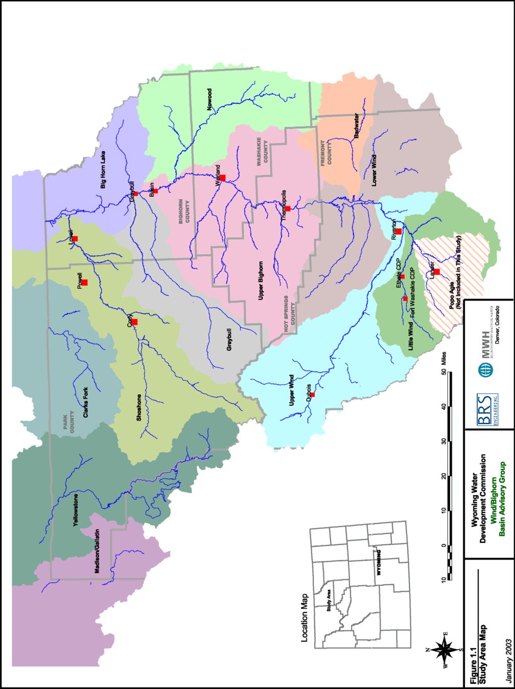
Figure 1-1. Study Area Map
1.1 Model Overview
The models are intended to simulate existing river operations for dry, average and wet year hydrologic periods. In general, existing operations are reflected in the historical operations within the study period. As discussed in the Task 3A/3B Technical Memorandum Surface Water Hydrology (MWH, 2002), this was the basis for selecting the study period, 1973-2001. In a few instances where existing conditions are different that either a portion or all of the historical conditions, special provisions in the data input and modeling calibration were required and are documented within the calibration section of this technical memorandum.
The primary data required for the spreadsheet models are streamflow, actual (or estimated actual) diversions, full supply diversions, irrigation returns and reservoir operations. For each of these, the data within the study period was reduced into dry, average and wet year data. The reduction of streamflow data, including the calculation of natural flow data for those tributaries that do not contain diversions, is described in the Surface Water Hydrology Technical Memorandum (MWH, 2002). Development and reduction of actual diversion data is discussed Technical Memorandum Irrigation Diversion Operation and Description (BRS, 2003) Task 2A Technical Memorandum Agricultural Water Use and Diversion Requirements (MWH, 2003a), while the estimation of actual diversion for those diversions without actual measurements is discussed later in this Technical Memorandum.
The model is run on a monthly timestep for the given calendar year of the hydrologic condition (dry, average, and wet). Starting reservoir levels are the same as the historical end-of-month contents on the last day for that hydrologic condition (i.e., the dry year model starting contents in January is the historical dry year end-of-month contents in December).
The basic model calculation procedure is shown in Figure 1-2. Natural flows for each main channel and tributary are either taken from gage data (preferred but not normally available) or estimated using the regional regression techniques as describe in the Task 3A/3B Technical Memorandum Surface Water Hydrology (MWH, 2002). Then, the incremental gains and losses are calculated for each reach. This is performed by locating the first downstream gaged node and constructing a .basin. containing all of the known upstream inflows, diversions and reservoir operations. The basins often contain many tributaries to the gaged node. Once the ungaged gains and losses are calculated, they are distributed to each reach within the basin by pro-rating the gains and losses based upon the reach.s contribution to the gage flow. Ungaged gains are applied at the top of the reach to allow for diversion, while the ungaged losses are applied to the bottom of the basin to allow diversion of computed inflows.
Once the ungaged gains and losses are calculated, a mass balance (or water budget) is computed at each node. At nodes other than storage nodes, the amount of flow available to the next downstream node is calculated as the difference between known inflows, such as tributary inflows, return flows, basin gains and imports, and outflows, such as diversions, basin losses and exports. At storage nodes, the losses due to evaporation and the gains/losses due to change in storage are included in the calculations. Diversions are limited to the lesser of the full supply diversion and the physical streamflow. The mass balance is performed from upstream to downstream for each node in the reach, and for each reach in the model.
Model output includes the following:
The model has been modified as explained in later sections of this technical memorandum to allow estimation of impacts on streamflow and diversions of various water projects, including Tribal Futures projects and storage projects. The model can also be modified to estimate impacts due to storage projects, instream flow water rights, or other water development projects.
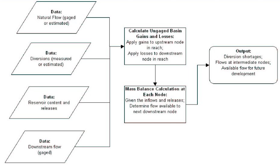 Figure 1-2. Generalized Model Flowchart
The limitations of the model should be noted:
1.2 Model Development
As with the previous river basin plans, the models for the Wind/Bighorn River basin plans were developed using Microsoft® Excel 97. All computations within the workbooks are performed using formulas written in the cells of the workbooks. The workbooks also contain macros that are used only for navigation between the various worksheets in the workbooks. The model calculations are completely automated so that when data is changed in any cell, the entire model is updated. The one exception is when data is shared between models. The procedures for sharing data between models is discussed in more detail later in this document.
As requested by WWDC, the models were developed for the novice Excel user. Basic proficiency in spreadsheet usage is required to view results and to make minor changes to input data and variables. However, to input additional nodes or reaches in the model, a more advanced level of proficiency is required. Interactive buttons have been placed throughout the spreadsheets to allow for easier navigation between the spreadsheets. All .tabs. and .row-column headers. within the model have been activated ad it was found that for most users, this information is useful to view. Also, due to the size and calculation time of the models, .manual calculation. has been selected as the calculation procedure. In this mode, model calculations are not performed until the users hits the .F9. key on the keyboard. Extreme caution should be exercised by those wishing to made construction changes to the model construction.
1.3 Model Structure and Components
Each of the models contains spreadsheets (or workbooks) consisting of several worksheets (or pages). Each worksheet either contains specific data related to the model, performs a related portion of the calculations, or contains output data. Consistent with the previous basin models, there are five basic types of worksheets, each containing a set of named worksheets.
The final main section of this technical memorandum contains programmers. notes. These notes are specifically targeted at those users who are seeking to make modifications to the model construction, such as adding nodes, analyzing alternatives or updating data.
Section 2 - Model Schematics
The physical structure of each model is represented in the river basin schematics and the reach schematics. Separate schematics have been developed for each model. The development of these schematics is discussed in the following paragraphs. Because of their size, the river basin schematics are included in the map pockets at the rear of this document, and labeled as Plates 1 through 12. The reach schematics are shown in Figure 2-1 through Figure 2-12.
2.1 River Basin Schematics
The river basin schematics are detailed link-node representations of the river basins. The schematics include nodes representing streamflow gages, natural flow nodes, diversion nodes, lumped diversion nodes, points of confluence and specific points of return flows if not already represented by a node. The nodes are connected by a series of links that represent the actual flow of water (normally in a stream) between the nodes. It should be noted that for visual clarity, the schematics are connected by straight links and are not to scale. Normally, the general flow direction through the schematic mirrors the actual flow direction, with north pointing towards the top of the schematic.
The following guidelines were used in developing the schematics:
River basin schematics were initially constructed by MWH, then sent to a list of schematic reviewers who had either volunteered or were selected based on their knowledge of the river basins. Comments were received from these reviewers and incorporated into the schematics as appropriate.
2.2 Reach Schematics
The reach schematics are simplified versions of the river basin schematics that are developed on a .reach. basis. Reaches are a group of nodes that represent an entire tributary or a portion of the main river. As discussed in later sections, the model calculations and water availability are generally performed and reported on a reach basis. The reach schematics are also used for navigational purposes within the model Graphical User Interface (GUI).
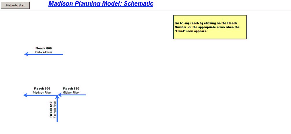 Figure 2-1. Reach Schematic - Madison/Gallatin Model
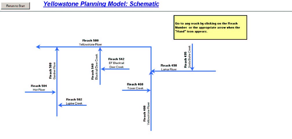 Figure 2-2. Reach Schematic - Yellowstone Model
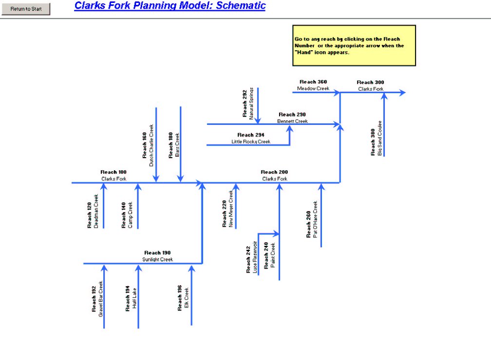 Figure 2-3. Reach Schematic . Clarks Fork Model
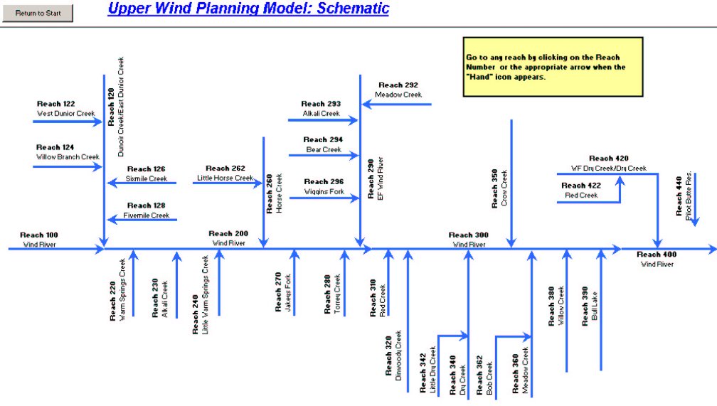 Figure 2-4. Reach Schematic . Upper Wind Model
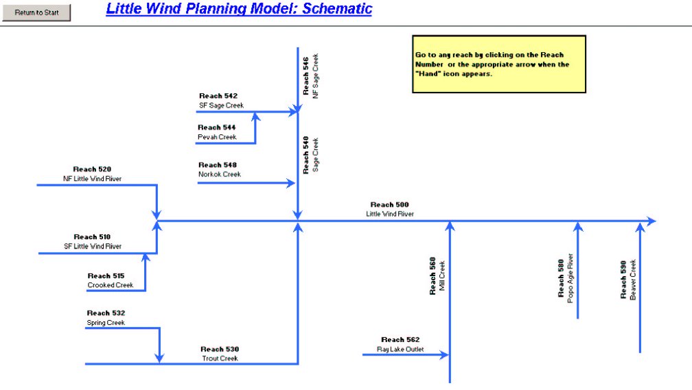 Figure 2-5. Reach Schematic . Little Wind Model
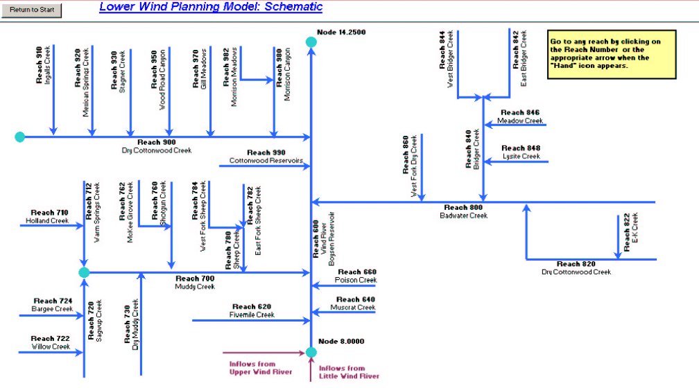 Figure 2-6. Reach Schematic . Lower Wind Model
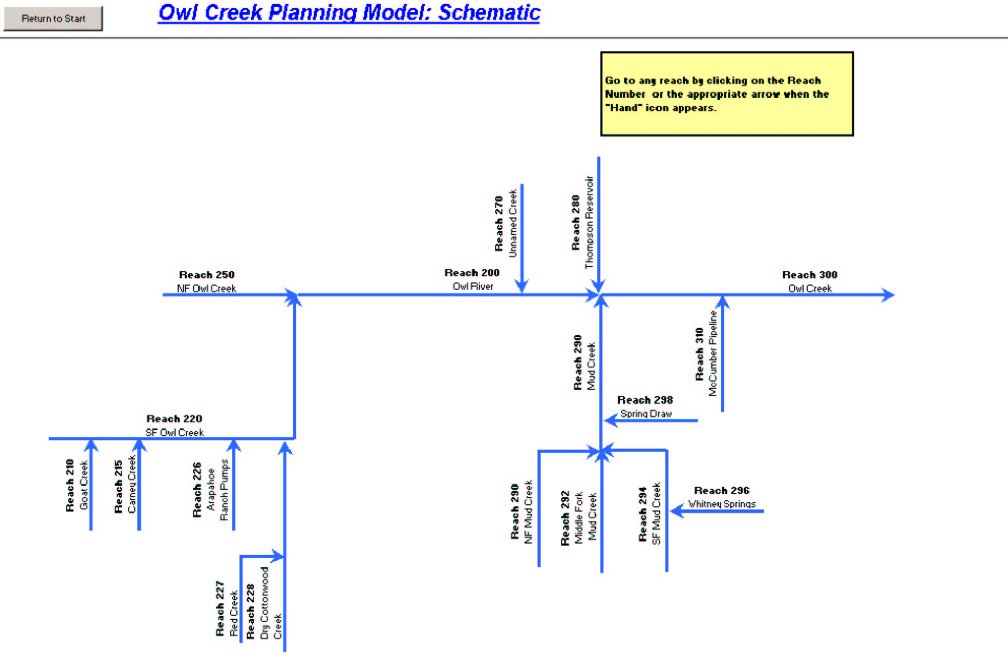 Figure 2-7. Reach Schematic . Owl Creek Model
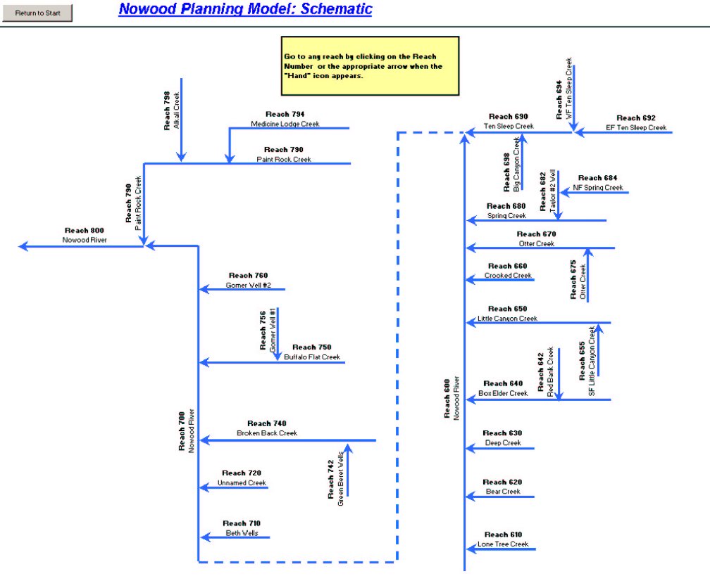 Figure 2-8. Reach Schematic . Nowood Model
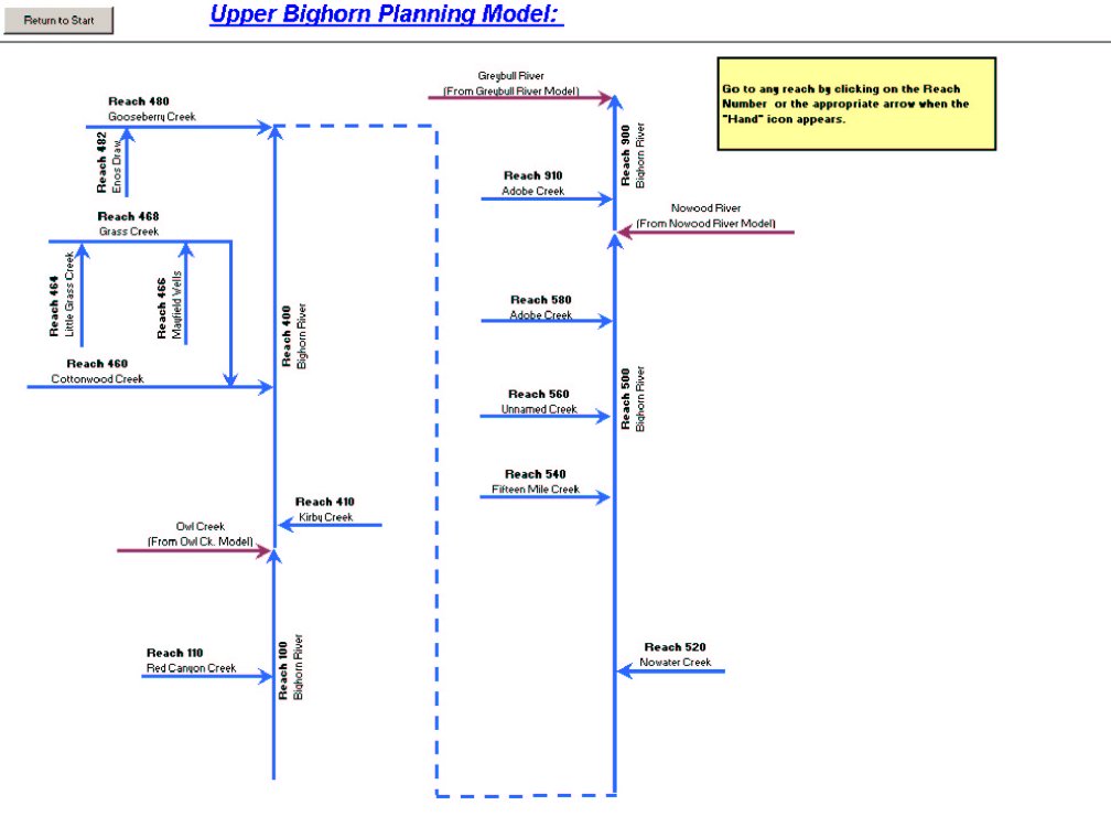 Figure 2-9. Reach Schematic . Upper Bighorn Model
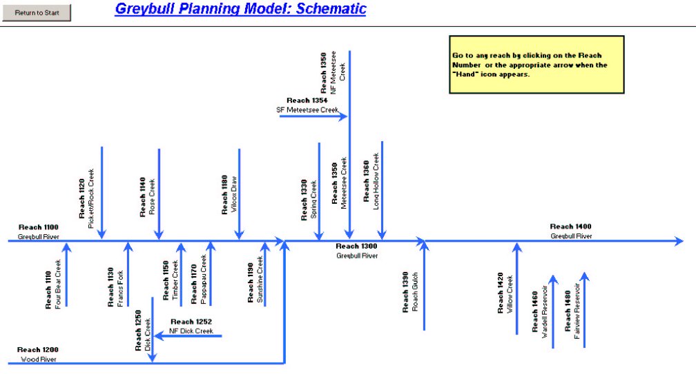 Figure 2-10. Reach Schematic - Greybull Model
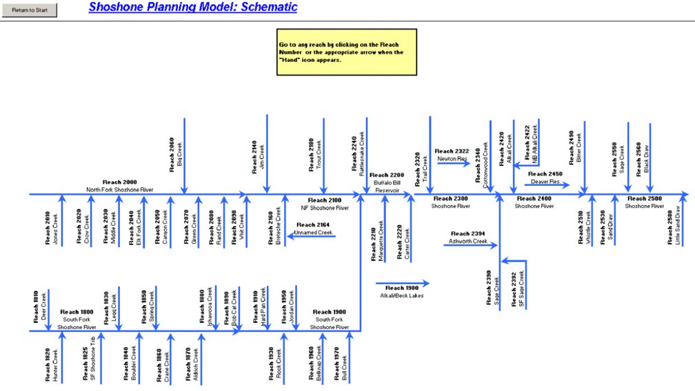 Figure 2-11. Reach Schematic - Shoshone Model
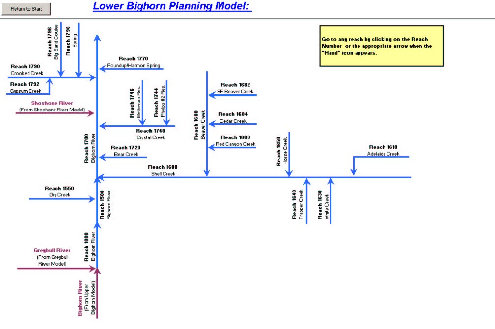 Figure 2-12. Reach Schematic . Lower Bighorn Model
Section 3 - Navigation Worksheets
The navigation worksheets are the primary components of the model Graphical User Interface (GUI). The GUI allows easier navigation between the different workbooks (or spreadsheet files) that make up the complete model, as well as easier navigation within each workbook. Each of the model GUIs worksheets, as well as the navigation to and from the calculation worksheets, are discussed in this section.
3.1 Main Model GUI
To start a sub-basin model, the user opens the main model spreadsheet. This workbook presents a GUI that allows the user to learn about the model structure, run a brief tutorial or navigate to the dry, normal and wet year models. As shown in Figure 3-1, the main model file is called $$$$$$_Model.xls, while the individual hydrologic year models are called $$$$$$_dry.xls, etc. (Note that in this figure and in the following text, $$$$$$ represents the name of an individual model. Figure 3-1 shows the Upper Wind model as an example.) The main workbook GUI is shown in Figure 3-2. The main model workbook does not perform any of the model calculations.
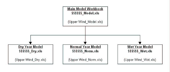
Figure 3-1. Typical Model Workbook Structure
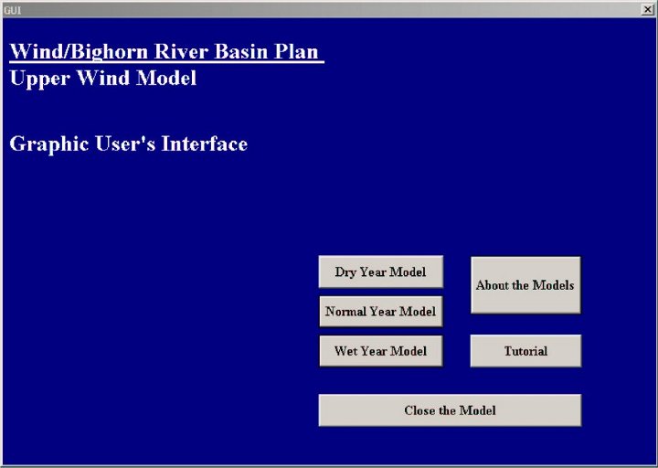
Figure 3-2. Main Model GUI
User Notes The following options are available from the GUI:
| Dry Year Model: | Opens the Dry Year Model workbook, |
| Normal Year Model: | Open the Normal Year Model workbook, |
| Wet Year Model: | Opens the Wet Year Model workbook, |
| About the ($$$$$$) Model: | Obtain information pertaining to the current version of the model, |
| Tutorial: | Opens a brief tutorial that describes the general structure of a spreadsheet workbook |
| Close the ($$$$$$) Model: | Closes all open workbooks. |
3.2 Central Navigation Worksheet
The central navigation worksheet is located in each of the dry, normal and wet year model workbooks, and is the worksheet that first appears when the individual model workbooks are opened. The central navigation worksheet allows the user to navigate to different areas of the workbook, and contains data regarding the reaches contained in the model. An example worksheet is shown in Figure 3-3.
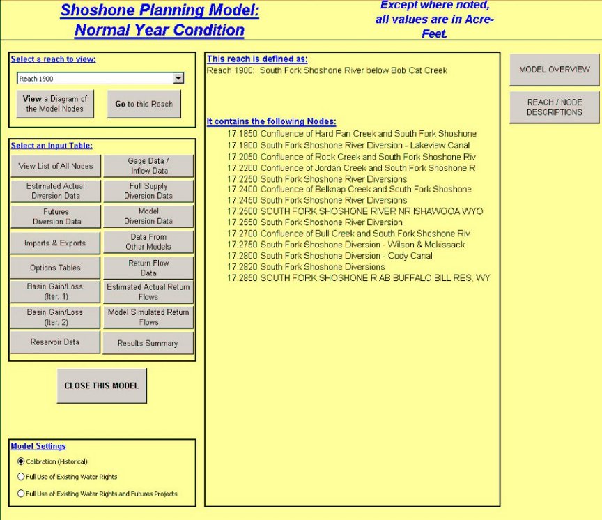 Figure 3-3. Central Navigation Worksheet
User Notes
This is the worksheet that first appears when the individual model workbooks are opened. In addition, nearly every other worksheet in the model has a button that allows the user to navigate back to this worksheet. The following buttons are located on this worksheet:
Reach Views:
| View a Diagram of the Model Nodes: | The sub-basin diagram (View a Diagram of the Model Nodes); |
| Go the this Reach: | Navigate to the reach worksheet shown in the pull-down menu; |
Input Tables:
| View list of all Nodes: | Navigate to the node list worksheet; |
| Gage Data/Inflow Data: | Navigate to the worksheet containing gage data and natural flow data; |
| Estimated Actual Diversion Data: | Navigate to the worksheet containing the actual diversion data and estimated actual diversion data for each node; |
| Full Supply Diversion Data: | Navigate to the worksheet containing full supply diversion data for each node; |
| Futures Diversion Data: | Navigate to the worksheet containing the diversion data including futures projects for each node; |
| Modeled Diversion Data: | Navigate to the worksheet showing the diversion data for each node used in the model run, which is based on the selected run type; |
| Imports & Exports: | Navigate to the worksheet containing imports & exports for each node; |
| Data From Other Models: | Navigate to the worksheet containing data imported from other models; |
| Options Tables: | Navigate to the worksheet containing optional data, such as irrigation return flow values and lag patterns. |
| Return Flow Data: | Navigate to the worksheet containing return flow locations and table values for each node; |
| Basin Gain/Loss (lter.1): | Navigate to the worksheet containing the first iteration of basin gain/loss calculations; |
| Estimated Actual Return Flows: | Navigate to the worksheet containing the actual return flow calculations. |
| Basin Gain/Loss (lter. 2): | Navigate to the worksheet containing the second iteration of basin gain/loss calculations; |
| Model Simulated Return Flows: | Navigate to the worksheet containing the model simulated return flow calculations. |
| Results Summary: | Navigate to the Results Summary worksheet that leads in turn to several summaries of output. |
Model Settings:
The model settings radio buttons select the run type as described by the buttons.
3.3 Summary Navigation
The summary navigation worksheets assist the user in navigating through the summary worksheets. A view of the summary navigation worksheet is shown in Figure 3-4.
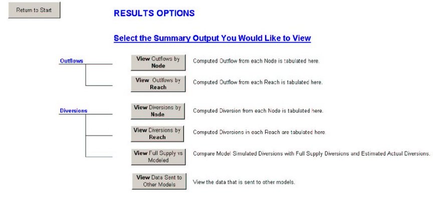 Figure 3-4. Summary Navigation Worksheet
3.3.1 User Notes
As shown in the figure, the worksheet is divided into two sections, outflows and diversions, which correspond to the summary worksheets. The following buttons are located on this worksheet.
| View Outflows by Node: | Navigate to the table in the outflows worksheet that contains a summary of outflows by node; |
| View Outflows by Reach: | Navigate to the table in the outflows worksheet that contains a summary of outflows by reach; |
| View Diversions by Node: | Navigate to the table in the diversions worksheet that contains a summary of diversions by node; |
| View Diversions by Reach: | Navigate to the table in the diversions worksheet that contains a summary of diversions by reach; |
| View Full Supply vs Modeled: | Navigate to the table in the diversions worksheet that contains a summary of the full supply versus modeled diversions for each node; |
| View Data Sent to Other Models: | Navigate to the worksheet that contains the data sent to other models. |
| Return to Start: | Navigate to the navigation worksheet. |
Section 4 - Data Input Worksheets
As shown in the river basin and reach schematics, the model performs calculations at reaches that represent physical points along the rivers and their tributaries. Natural flow nodes, gage nodes, diversion nodes and reservoir nodes all contain input data to the model. The following sub-sections review the data entry worksheets for each of the node types.
4.1 Master List of Nodes
The Master List of Nodes worksheet presents a master list of all nodes included in the models. In addition, the worksheet contains data indicating the reach in which the node is contained. The nodes correspond to those nodes shown on the reach and river basin schematics. A comprehensive list of nodes is shown in the appendices. A sample of the worksheet is shown in Figure 4-1.
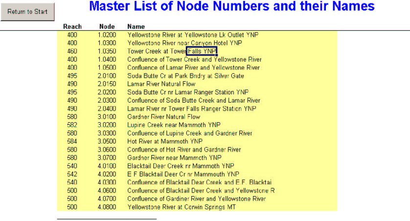 Figure 4-1. Master List of Node Worksheet
Engineering Notes
The nodes and reaches were developed based upon the locations of data, locations of diversions and key tributary inflows. The node number system was developed to allow insertion of additional nodes as the model continues to be used for other purposes. Nodes are generally numbered from upstream to downstream. Similarly, reaches were designated and numbered to allow insertion of additional reaches without the need to renumber existing reaches. In general, those reaches labeled on the even 100.s are main channels. Those reaches labeled in the 110.s are tributary reaches while reaches labeled in the 111.s are secondary and tertiary tributary channels.
User Notes:
The Master List of Nodes allows the User to view a simple, comprehensive listing of all nodes within the model, organized by reach and node number. This master list governs naming and numbering conventions on many worksheets, so changes to the list must be done with great care. Many of the calculations within the spreadsheet are dependent on the proper correlation of node names and numbers.
4.2 Gage and Natural Flow Data
The gage and natural flow data contains the actual and estimated gaged flow data and natural flow data. Gage data is from USGS, SEO or USBR gaging stations that was filled based on regression equations when necessary for the study period. The data was then reduced to dry, normal and wet year flows. Natural flow data is necessary at the headwaters and tributary inflows where gage data does not represent natural flows. These flows were developed using regional basin regression equations that are dependent upon various basin characteristics. The development of this data is detailed in the Task 3A/3B Technical Memorandum Surface Water Hydrology (MWH, 2002). A sample of the worksheet is shown in Figure 4-2.
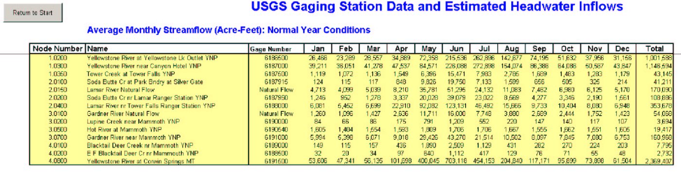 Figure 4-2. Gage and Natural Flow Worksheet
Engineering Notes
The development of this data is detailed in the Task 3A/3B Technical Memorandum Surface Water Hydrology (MWH, 2002).
User Notes
The Gage Data Table presents the average historical monthly gage and natural flow data for each hydrologic condition used in the model. Only the data pertaining to the hydrologic condition being modeled are included in each respective model. In addition, this worksheet only contains nodes that have hydrologic data. Nodes that do not contain hydrologic data are not included in this list.
4.3 Diversion Data
The Wind/Bighorn model can be run in three different modes:
The model utilizes the appropriate data associated with these three modes. Each set of data is stored on a separate worksheet, with a fourth worksheet used to store the set of data actually used by the calculations.
The Wind/Bighorn basin planning model simulates diversion in two different steps.
As shown on the basin schematics, diversions were generally divided into two categories: those greater than 10 cfs and those less than 10 cfs. Those diversions that are greater than 10 cfs were individually modeled while those less than 10 cfs were modeled as .lumped. diversions. All diversions were explicitly modeled . the model considered either their actual diversion or an estimate of their actual diversion, their required diversion and their return flow locations. Some small diversions (those less than 10 cfs) are modeled individually because it is the only diversion located on a tributary, because it is the only diversion between two other model nodes or because it is the only diversion in a significantly long reach of the river. Diversion data and estimated diversion data were divided into dry, average and wet years. Required diversion volumes were not separated into dry, average and wet years.
Municipal diversion data is also included on these spreadsheets. For those municipalities that use surface water diversions, both diversions and return flows were included in the model. For those municipalities that use groundwater, only surface water return flows were included in the model. Any groundwater depletions caused by pumping or groundwater returns from outdoor water use are implicitly calculated in the gain-loss portion of the model.
Data regarding diversions are shown on three worksheets: the Estimated Actual Diversion Data (Historic Diversions) worksheet and Full Supply Diversion Data (Ideal Diversions) worksheet, and the Futures Diversion Data worksheet. The Model Diversion Data worksheet compiles the correct data for use in the simulation based on the run type. The worksheets are essentially the same in the appearance and data entry, except that the Estimated Actual Diversion Data worksheet contains two intermediate tables that allow adjustment of the estimated data based upon the hydrology. Samples of the worksheets are shown in Figure 4-3, Figure 4-4, Figure 4-5 and Figure 4-6.
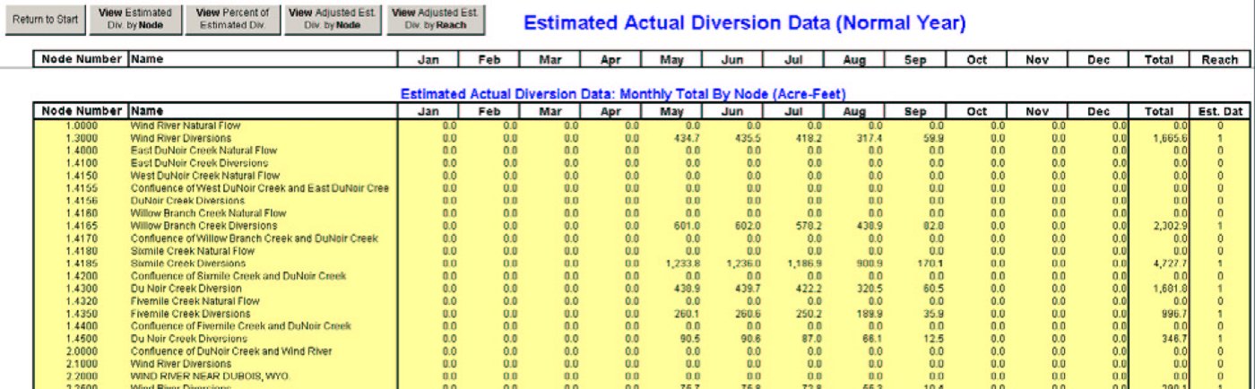 Figure 4-3. Estimated Actual Diversion Data Worksheet . Data
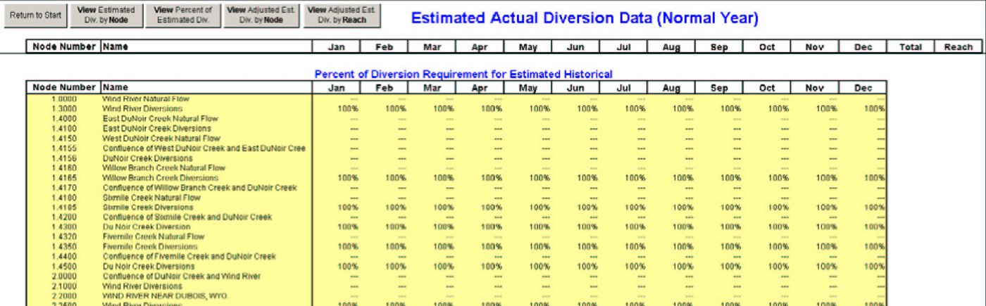 Figure 4-4. Estimated Actual Diversion Data Worksheet . Percent of Diversion Requirement
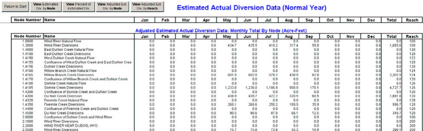 Figure 4-5. Estimated Actual Diversion Data Worksheet . Adjusted Estimated Actual Diversion Data by Node
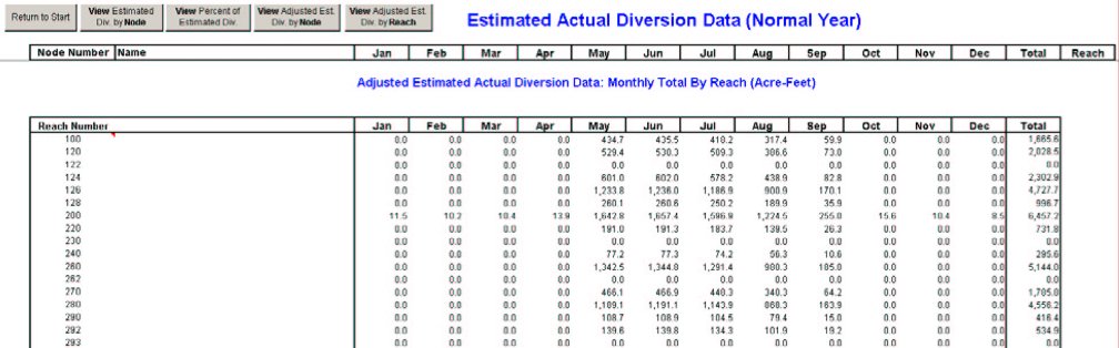 Figure 4-6. Estimated Actual Diversion Data Worksheet . Adjusted Estimated Actual Diversion Data by Reach
Engineering Notes
Collection of agricultural diversion data is discussed in the Technical Memorandum Irrigation Diversion Operation and Description (BRS, 2003).
The estimated consumptive irrigation requirement (CIR), duration of irrigation, actual historic diversions and full supply diversions is described in the Task 2A Technical Memorandum Agricultural Water Use and Diversion Requirements (MWH, 2003a).
Municipal diversions were taken from the Technical Memorandum Municipal Basin Water Use Profile (LA, 2002). Values reported in this memorandum represent the consumptive use portion as well as the entire historical diversion amount of the municipal diversions. No attempts were made to develop dry, normal and wet year municipal diversions. There were no industrial uses significant enough to be modeled. For those municipalities using groundwater, only surface water returns were included in the model.
User Notes
The diversion data worksheets contain only input data for each node for an average dry, normal, or wet year. Note that all nodes are listed in the tables, even if no diversions occur at them. At the top of the worksheets are buttons that will take the User to the table summarizing the total monthly diversions in each reach. With the exception of these summary tables, no computations occur within these worksheets. It should be noted that both node number and node name are required to be manually input by the user.
4.4 Return Flows
To provide more expedient data entry and to allow easier comparison between return flow values, in the Wind/Bighorn River basin models, return flows are entered on a separate worksheet called the .Return Flow Data. worksheet. The return flow worksheet documents the spatial and temporal return flow patterns, as well as the efficiency patterns for each node in the model. A sample of the worksheet is shown in Figure 4-7.
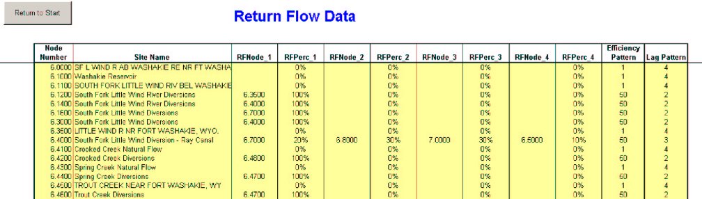 Figure 4-7. Return Flow Data Worksheet
Engineering Notes
Spatial return flow patterns are estimated based upon the location of the irrigated lands associated with each node and the next downstream node. More accurate information was available in some cases, where previous information was available or where water users had information.
Efficiency patterns were developed based on available existing data. These data sources included the Wind River On-Farm Report, the Shell Creek report and the Water Use profiles report. Efficiency patterns can vary greatly from diversion to diversion, and have a significant impact on the amount of water that is required for a diversion. However, it is not the intent of this study to provide an in-depth analysis of efficiencies. Therefore, only data available from previous studies was used in the analysis.
Lag patterns for diversion return flows are a key element in the model calibration process. Initially, lag patterns are set so that all return flows return in the same month that they are diverted. Then, through the calibration process, lag patterns are modified. A standard set of lag patterns has been developed, and is discussed in the .Options. worksheet portion of this document.
User Notes
The return flow spreadsheet contains information for each node regardless of whether it contains diversions. In order for the Excel calculations to perform correctly, the return flow percentage columns must contain a value. Therefore, if the node does not have return flows, a value of 0% must be entered for the return flow percentage. The table does not need to have return flow nodes entered in each cell.
During the calibration process, any changes to return flow lag patterns are made in this worksheet.
4.5 Import and Export Data
Imports and exports pertain to the physical import or export of water from one basin to another through a transbasin diversion facility. Imports and exports should not be confused with simple data transfers between models, as further described below. Flows available for export were determined using the same methodology for other diversions as described in the Task 3A/3B Technical Memorandum Surface Water Hydrology (MWH, 2002). A sample of the worksheet is shown in Figure 4-8.
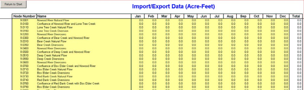 Figure 4-8. Import/Export Data Worksheet
Engineering Notes:
The only imports or exports modeled in the Wind/Bighorn basin planning models occur in the Greybull and Shoshone models. Flow from the North Fork of Meteetsee Creek in the Greybull Model is exported to Foster Reservoir in the Sage Creek basin of the Shoshone Model.
User Notes:
The Imports/Exports Table summarizes the monthly imports to or exports from other basins. As noted above, only the Greybull River/Shoshone River imports were explicitly modeled as such. However, the node water balance tables in the Reach/Node Worksheets are set up to incorporate imports to or exports from any node.
4.6 Reservoir Data
Although referred to in the model as the Reservoir Evaporation Loss worksheet, the worksheet contains all data for reservoirs within the model, including evaporation and precipitation data that are used to calculate net evaporation, historical end-of-month contents, historical releases and the stage-area-capacity curves. The volume of water lost to the system through evaporation is calculated by interpolating the water surface area for each reservoir based on the end-of-month contents. This evaporation data, as well as releases from the reservoir, are used in the reach mass balance calculations. A sample of the worksheet is shown in Figure 4-9.
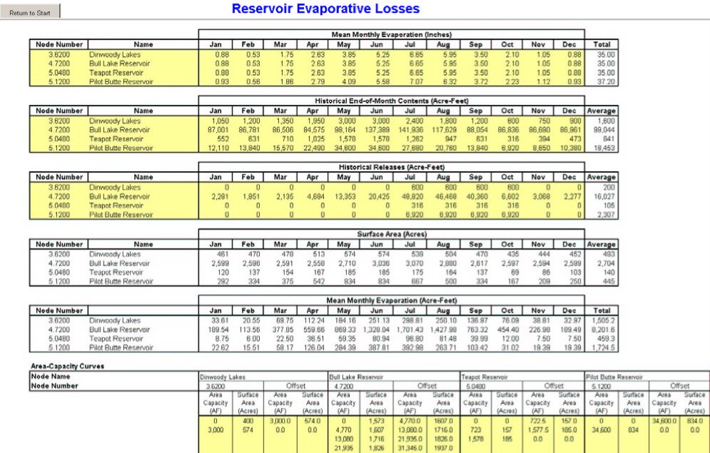 Figure 4-9. Reservoir Data Worksheet
The model explicitly models all reservoirs greater than 500 acre-feet. Any reservoirs less than 500 acre-feet are implicitly included in the gage flows and gain-loss calculations. Historical storage and release data was not available for many of the reservoirs. In addition, not all reservoirs contain stage-area-capacity curves.
Engineering Notes
Monthly gross evaporation, precipitation data and area-capacity data for each of the modeled reservoirs was obtained from the Technical Memorandum Water Use From Storage (LA, 2002).
Historical end-of-month reservoir contents, diversions, and releases were obtained from the water users or the US Bureau of Reclamation. Dry, normal and wet year end-of-month contents were determined for each reservoir based upon the same methodology as described in the Task 3A/3B Technical Memorandum Surface Water Hydrology (MWH, 2002).
For those reservoirs that did not contain a rating curve, the rating curve was assumed as a two-point curve, which assumes a linear interpolation between empty and full stage-storage.
Calibration Notes
Because reservoir data was not available for a majority of the reservoirs, initially, estimated contents were assumed for each of the reservoirs based on filling in the spring months and drawdowns later in the summer. Then, releases and the subsequent end-of-month contents were modified so that they were reasonably calibrated with the gain-loss calibrations.
User Notes
Monthly gross evaporation (inches) and total precipitation (inches) data are included in the table. The net evaporation in inches is then calculated within the worksheet. The end-of month surface area is calculated from the area-capacity table and used to determine the mean monthly evaporative loss in acre-feet. As with other tables in the model spreadsheet, cells that require an entry are highlighted in yellow.
4.7 Irrigation Return Patterns and Lag Tables
Two tables are shown on the Options worksheet and are described as follows:
A sample of these two tables is shown in Figure 4-10.
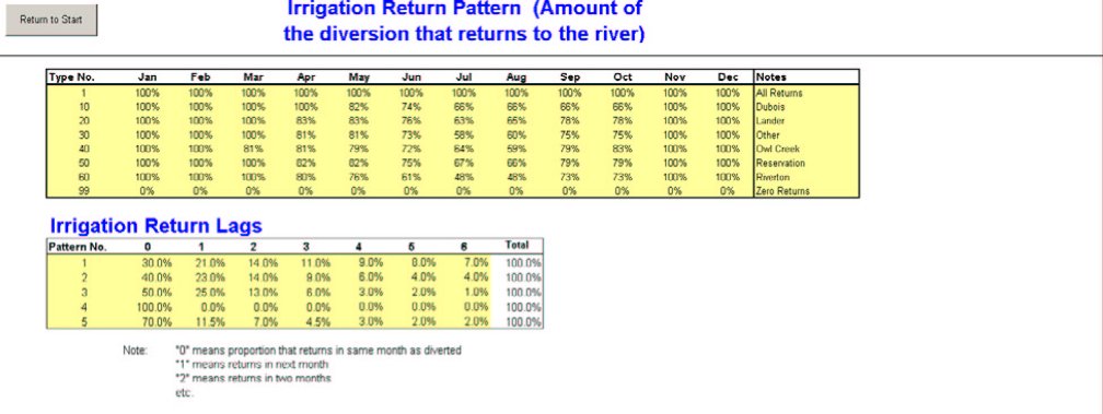 Figure 4-10. Irrigation Return Patterns and Lags
Engineering Notes
The unused, or inefficiency portion of diversions is returned to the river over the course of one or more months either by direct surface runoff, or through the alluvial aquifer. For modeling purposes, an estimate must be made of amount, location, and timing of returns. The Options Table addresses amount and timing of return flows. The points of diversion (service area) GIS theme contains the information designating the Return Pattern and Return Lags for each model node.
The Irrigation Return Pattern table provides the monthly return fractions (inefficiencies) for every diversion in the model. One pattern is characterized by zeros in all months, which is applicable to all intra-basin diversion nodes, such as the diversion of water through Dinwoody Canal, which is a feeder canal to the Upper Bench Canals. Monthly efficiencies for irrigation diversions were developed by comparing historical diversion records to the theoretical maximum diversion requirement (based on CIR) as discussed in the Task 2A Technical Memorandum Agricultural Water Use and Diversion Requirements (MWH, 2003a). The return flow fraction is defined as (1.0 . Efficiency).
Lags for irrigation diversions were patterned after similar previous projects and adjusted based on the type of irrigation system defined in the irrigated lands mapping (i.e. conventional irrigation systems as opposed to spreader dikes or intermittent diversions from ephemeral streams). Irrigation Return Lags for municipal nodes were set to 100 percent during the month of diversion.
Calibration Notes
Efficiencies and return lags are an important step in the calibration process. The efficiencies and return lags initially selected were further calibrated to fit the conditions of the sub-basins using the magnitude and monthly pattern of the Ungaged Basin Gain/Loss term as a reasonableness check.
User Notes
The Options Tables incorporate the information used in the computation of irrigation return flow quantities and their timing. The data in the first table, .Irrigation Return Patterns,. consist of the percentages of water diverted which eventually will return to the river and be made available to downstream users.
The second worksheet table, .Irrigation Return Lags., controls the timing of these returns. Flows diverted in any month can be lagged up to six months beyond the month in which they are diverted. An example pattern is:
| Month | 0 | 1 | 2 | 3 | 4 | 5 | 6 |
| Percent | 30 | 21 | 14 | 11 | 9 | 8 | 7 |
By way of example, for a diversion occurring in July, 30 percent of the Total Irrigation Returns (i.e., that portion not lost to consumptive use, evaporation, etc.) will return in July, 21 percent in August, 14 percent in September, 11 percent in October, 9 percent in November, 8 percent in December, and the remaining 7 percent will return in January.
4.8 Data Transfer From Other Models
Because of the size of the Wind and Bighorn basins, the river basins were separated into several sub-basin models. As a consequence, there are several occasions when data is required to pass between the models. Examples of this include:
These types of interactions differ from imports and exports because imports and exports between basins are intended to model physical transbasin export from one basin to another. Data transfer between models is necessary when data must be transferred simply because the basins have been subdivided into one or more models.
A sample of the data transfer worksheet is shown in Figure 4-11.
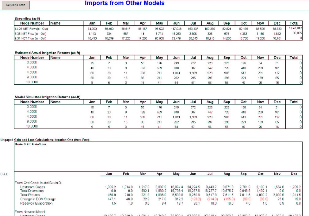 Figure 4-11. Upstream Flows From Other Models Worksheet
Engineering Notes
This worksheet does not perform any calculations.
User Notes
Data on this worksheet is linked directly to the spreadsheet from which it originates. Therefore, if changes are made in the source worksheet, then the links must be updated. In addition, if any lines are inserted or deleted, the links must be relinked to ensure that the correct data is imported.
When any of the sub-basin models with links is opened, it will ask the user if the links should be updated. If the user is only using the model to investigate impacts with the model sub-basin, then the links do not need to be opened. However, if the user is determining impacts of changes to the model on all downstream users, then the links need to be updated when opening the downstream sub-basin models.
Section 5 - Model Computation Worksheets
The model computation worksheets are the heart of the sub-basin models. The primary model calculations are performed within these worksheets, including the calculation of return flows, the calculation of ungaged basin gains and losses, and the water balance for each reach.
5.1 Irrigation Returns
The unused portion of a headgate diversion either returns to the river as surface runoff during the month it is diverted, percolates into the alluvial aquifer or deep percolates into sub-alluvial aquifers. The portion that percolates into the alluvial aquifer returns to the river through sub-surface flow, but generally lags the actual diversion by several months. In general, unless there is information that is contradictory, it is assumed that all sub-surface return flows are to the alluvial aquifer and thus return to the river. The location of the return flow.s re-entry to the surface water system is an important factor in modeling the basin, and depends on the specific topography and layout of the irrigation system. The location of irrigation return flows were determined through the irrigated lands mapping task and are specified as a GIS attribute for each irrigated service area.
There are two Irrigation Return worksheets:
Each of these Irrigation Return worksheets has three tables and are described as follows:
1. Calculates the amount of return flow resulting from each month.s diversion at each node, and distributes it in time and place according to the information in the Options Table. 2. Figure 5-1 shows the calculation tables for each return flow worksheet.
2. Table tabulates all the incoming return flows for each month at each node, from the various sources. This table produces the return flow component of inflow at each node.
3. Summarizes return flows by reach.
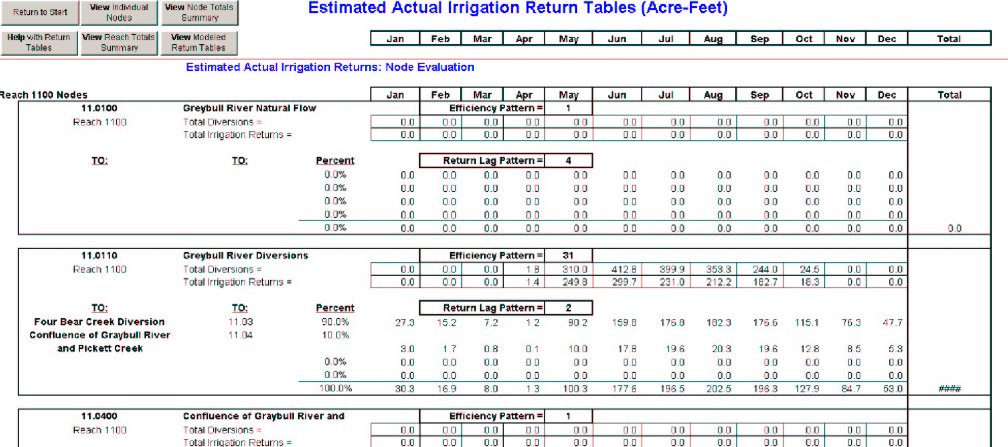 Figure 5-1. Estimated Actual Returns Worksheet
Engineering Notes
The following describes the terms and calculation procedures found in the irrigation return flow worksheets.
Efficiency Pattern: The value entered here is used to look up the Irrigation Return Pattern found in the Options Table. These values are referenced from the return flow worksheets.
Total Diversions: Estimated Actual Return Flows worksheet: values are referenced from the Estimated Actual Diversion Data input worksheet.
Model Simulated Return Flows worksheet: values are referenced from the .Summary of Diversion Calculations: By Reach. table on the Diversion Summary worksheet.
Total Irrigation Returns: These values are computed by multiplying the Total Diversions by the selected Irrigation Return Pattern for the month. For example, for a month with Total Diversions of 1000 acre-feet and an irrigation return fraction of 80%, the Total Irrigation Returns from that diversion for that month will be 800 acre-feet.
Return Pattern: The value entered here is used to look up the Irrigation Return Lag found in the Options Table. These values are referenced from the return flow worksheets.
To and Percent: This feature allows the User to define the node(s) in the model where irrigation returns will return and in what percentages. These values are referenced from the Return Flow worksheet.
Irrigation Returns: Node Totals Table: This table lists all of the irrigation returns that have been directed to each Node and provides their sum.
Irrigation Returns: Reach Totals Table: This table lists all of the irrigation returns that have been directed to each Reach and provides their sum.
User Notes
This worksheet computes the return flows from irrigation diversions. The User should modify only those cells highlighted in yellow. In general, the user will not modify values on this worksheet. It has been designed to be .self-computing. wherein values are referenced from other worksheets, primarily the Irrigation Diversion worksheets and the Return Flow worksheets.
Buttons at the top of the worksheet take the User directly to each of the three tables in the Irrigation Return Worksheet.
View Individual Nodes: takes the User to the first table, which calculates return flows from each node and distributes them in time and place.
View .Node Totals. Summary Table: takes the User to the second table, the Node Totals Table.
View .Reach Totals. Summary Table: takes the User to the Reach Totals Table.
5.2 Gain-Loss Calculations
The sub-basin models simulate the major inflows, storage facilities, diversions and other major elements of the river basin system. However, many more minor elements of the river basin system, such as small tributaries, small reservoirs, stock ponds, groundwater accretions/depletions, etc., are not explicitly included in the schematics or in the computer simulation of the physical system. To account for these elements in the model, their impacts are estimated through gain-loss calculations between known points of flow (i.e. streamflow gage nodes, natural flow nodes or reservoir releases). These impacts are then added back into the reaches represented in the model. These ungaged gains and losses account for all water in the budget that is not explicitly accounted for and includes ungaged tributaries, groundwater/surface water interactions, or any other process not explicitly modeled. Two iterations are performed for historical and simulated flows. Samples of each calculation are shown in Figure 5-2. Calculations are summarized in the gain-loss summary tables, which are shown in Figure 5-3.
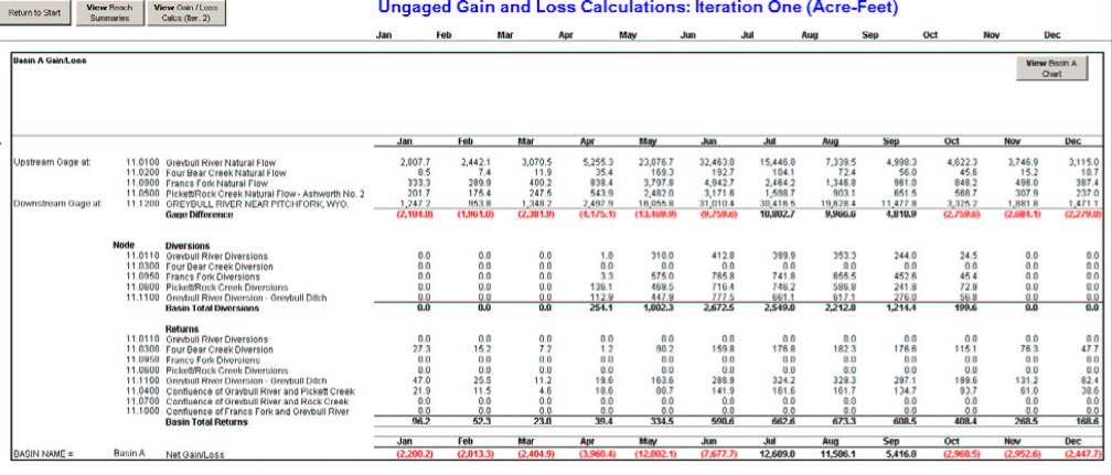 Figure 5-2. Ungaged Gain-Loss Calculations Iteration 1
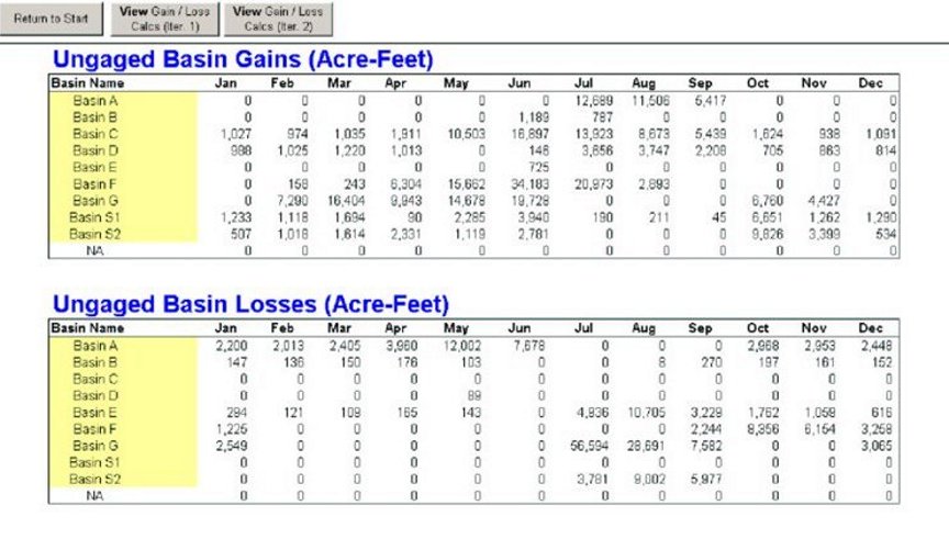 Figure 5-3. Gain Loss Summary Worksheet
Engineering Notes
Ungaged gains and losses are computed between gages using a water budget approach as described in the following equation:
Qgain = {Qdownstream . ∑Qupstream} + ∑Qdiversions . ∑ Qreturn flows . Δ EOM Storage + QEvaporation
All terms are supplied from the Input Worksheets, the Computation Worksheets, or the Summary Worksheets. Each gain-loss calculation is divided into a basin. Basins are defined by a gaged downstream node. Then, each known flow upstream of that node (gaged flows and natural flows), diversions, return flows and storage contents are used according to the equation above.
Calibration Notes
Two computational iterations are performed in establishing the ungaged gain/loss, with the following differences:
Iteration 1 - Uses the Estimated Actual Diversion Data and Historical Return Flows
Iteration 2 - Uses the Model Simulated Diversions and Model Return Flows.
The second iteration accounts for reductions in return flows resulting from diversion shortages and is necessary to achieve closure in the water balance calculations. Basin gains are equated to positive values, while basin losses are equated to negative values. The basin gain/loss charts are used to visually verify the reasonableness of the gain/loss pattern and magnitude. Model assumptions, input data, and schematic representations of the physical system were adjusted as necessary until the magnitude and monthly distribution of the gain/loss term appeared reasonable given the inherent limitations of the model and data deficiencies.
User Notes
The worksheet uses positive values from iteration one as Basin Gains and negative values from iteration two as Basin Losses. Mathematical closure in the water balance calculations is accomplished through adjustments made in the second iteration.
Basin Summary . takes the user to the Basin Summary Tables
View Basin $ Chart . allows the user to view the chart for that basin. $ is the Basin alphanumeric number.
5.3 Reach Water Balance Calculations
The water balance at each node is contained in the Reach Water Balance worksheets. Each node is represented in the spreadsheet by an inflow section, which includes inflow from the upstream node, irrigation returns, ungaged gains, and imports, if applicable; and an outflow section, which includes ungaged losses and diversions, if applicable. Storage nodes have the additional gains/losses due to storage releases or diversions, and losses due to evaporation. The algebraic sum of these flows is then the net outflow from the node. A sample of a non-storage node calculation table is shown in Figure 5-4, while a sample of a storage node calculation is shown in Figure 5-5.
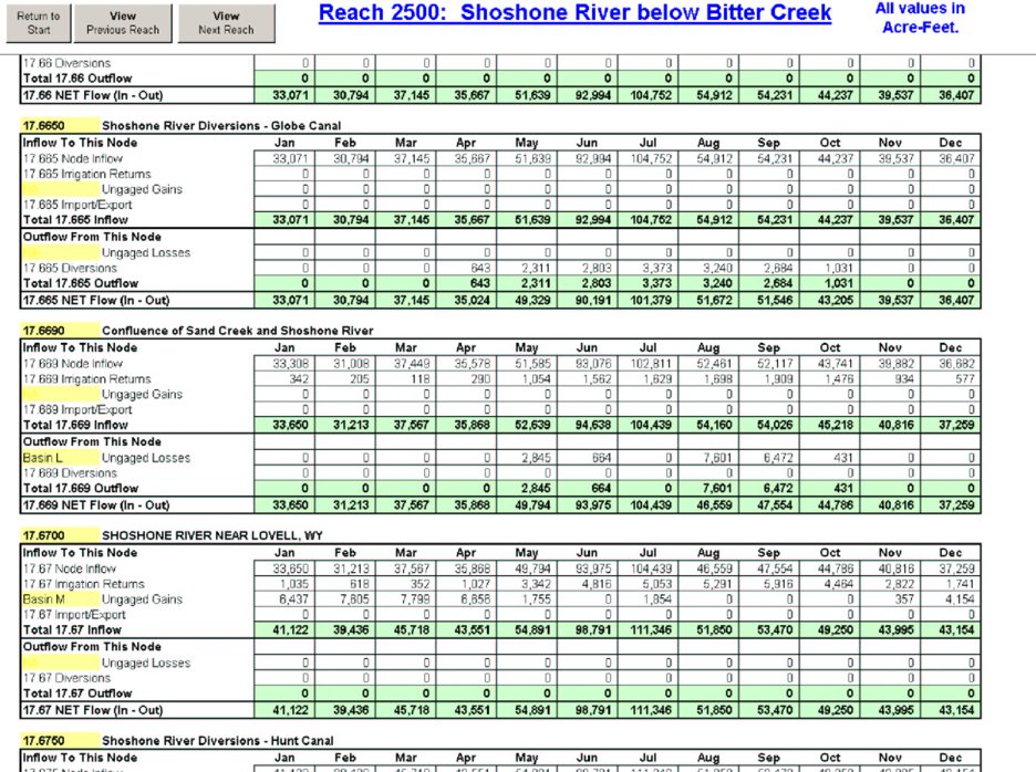 Figure 5-4. Reach Water Balance Worksheet
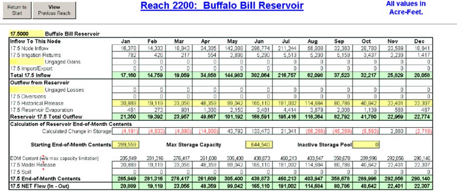 Figure 5-5. Reach Water Balance Worksheet - Reservoir Node
Engineering Notes
This is the heart of the spreadsheet model where water budget calculations are performed for each node represented in the model. Water balance is maintained in each river reach through the use of the Ungaged Basin Gain/Loss term. The total basin gain or loss is pro-rated based upon the known contribution of the particular reach to the overall river flow. Basin gains are added to the most upstream node on the reach while basin losses are accounted for at the node just upstream of the most downstream gage for the basin. This allows full diversion of the ungaged gain/loss by diversions within the reach.
The calculations are a mass balance at the node. The following equation describes the calculation:
where:
For nodes that have flow data, the node inflow is the flow data. Otherwise, this is the sum of the upstream node (or nodes if the node is a junction node).
At reservoir nodes, simulated end-of-month contents is also calculated. The following equation is used in the calculations:
Seom = Seom-previous + Qinflows . Qmodel releases . Evap . Qdiv . Qungaged losses
Obviously, end-of-month storage is limited to the actual storage contents of the reservoir. It should be noted that to avoid iterating between start-of-month and end-of-month contents to calculate evaporation, the historical or estimated historical evaporation is used for the evaporation term.
User Notes
The Node Tables compute the flow available to downstream users (NET flow) using a water budget approach.
The nodes must be organized in an upstream-to-downstream order within each reach. Diversion demands at each node are referenced from the Full Supply Diversion Data worksheet. Model simulated diversions are the lesser of full supply diversion requirements and available flow. In the event that the full supply demand cannot be met, a warning is provided to inform the User that the diversion has been shorted.
The following subsections contain miscellaneous notes about specific nuances within the Reach/Node tables in the six sub-basin models. See the .Model Node Map. and Node list within each model for the locations of the reaches and nodes discussed below.
Madison/Gallatin Model
Yellowstone Model
Clarks Fork Model
Upper Wind Model
Little Wind Model
Lower Wind Model
Upper Bighorn Model
Owl Creek Model
Nowood Model
Lower Bighorn Model
Greybull Model
Shoshone Model
Section 6 - Results Worksheets
The outflow worksheets allow the model user to view summarized output from the model, either by node, reach or overall model. The output worksheets simply tabulate information as calculated in other worksheets.
6.1 Outflow Summary Worksheet
The outflow summary worksheet presents the monthly outflow of each node and reach in the model as calculated in the reach calculation worksheets. Two sets of tables are shown on this worksheet. The first set of tables shows the outflow for each node in the model, grouped by reach. The second table summarizes this information for each reach. The reach outflow table is subsequently used to perform the available surface water calculations as detailed in Task 3D Technical Memorandum Available Surface Water Determination. (MWH, 2003b). A view of the worksheet is shown in Figure 6-1.
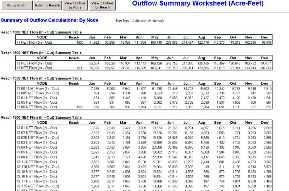 Figure 6-1. Outflow Summary Worksheet, Reach Tables
6.2 Diversion Summary Worksheet
The diversion summary worksheet presents the summary of diversion calculations for each node in the model as calculated in the reach worksheets. The diversion summary worksheet contains three sets of table. The first set of tables summarizes the simulated diversion for each node, grouped by reach. A sample of this table is shown in Figure 6-2. The second table summarizes the simulated diversions for each reach. The third table presents a summary of modeled versus full supply diversions. A sample of this worksheet is shown in Figure 6-3.
 Figure 6-2. Summary of Diversions by Node Table
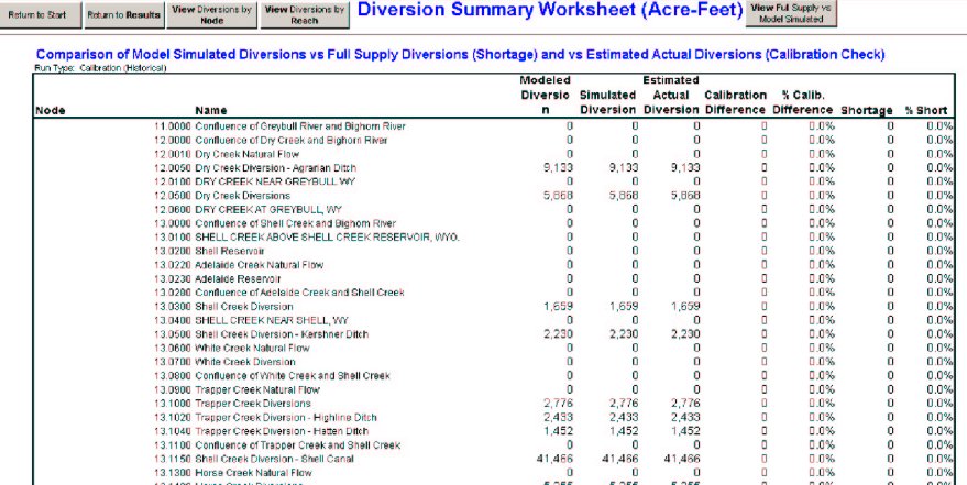 Figure 6-3. Diversion Summary Worksheet, Diversion Comparison Table
User Notes
The following definitions apply to the calculations shown in the diversion comparison table.
| Modeled Diversion | The total annual full supply diversion as given in the Full Supply Diversion spreadsheet. |
| Simulated Diversion | The total annual calculated diversion from the reach calculations. |
| Estimated Actual Diversion | The total annual diversion as given in the Estimated Actual Diversion spreadsheet. |
| Calibration Difference and Percent Calibration Diff. | The calibration difference is the Estimated Actual Diversion minus the Modeled Diversion. This value gives an indication as to how close the model simulates historical diversions. Previous River Basin Planning reports have considered values within 35 percent to be considered reasonable, with some values greater than 35 percent primarily due to a lack of information. There are several reasons for the variation between simulated and modeled diversions.
|
| Shortage Percent Shortage | The difference between Full Supply Diversions and Model Simulated Diversions. |
6.3 Data Transfer to Other Models
This worksheet is similar to the Upstream Flows from Other Models worksheet. Because of the size of the Wind and Bighorn basins, the river basins were separated into several sub-basin models. As a consequence, there are several occasions when data is required to pass between the models. Examples of this include:
1. When a downstream model requires data at the confluence with another model;
2. When diversions occur in one model and the return flows return to another model;
3. When basins used for basin gain/loss calculations encompass more than one model.
These types of interactions differ from imports and exports because imports and exports between basins are intended to model physical transbasin export from one basin to another. Data transfer between models is necessary when data must be transferred simply because the basins have been subdivided into one or more models.
A sample of the data transfer worksheet is shown in Figure 6-4.
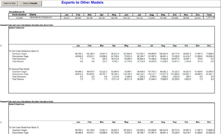 Figure 6-4. Exports to Other Models Worksheet
User Notes
Data on this worksheet is linked directly to the spreadsheet from which it originates. Links between models have been maintained as dynamic links. If changes are made to this model, then the data needs to be updated to models that are affected by the exports.
Section 7 - Calibration
Model calibration is required to adjust input parameters so that the model best matches real conditions. The Wind/Bighorn sub-basin models are full simulation models, wherein flow at each gage is simulated based on system inflows and losses. The one exception to this rule is reservoirs, which take into account historical contents and releases when calculations are made.
Two measures were primarily used for calibration of the models
Several input parameters were adjusted to most fully meet the calibration measures described above. These include:
Normally, because ungaged gains and losses are part of the model, the historical and simulated flow should match very closely. However, because of the reservoir calculations (especially for reservoirs with estimated data), not all basins are perfectly calibrated. In addition, because the model does not .look downstream. to see if all diversion requirements are met, the model basically .resets. itself at each mainstem reservoir.
The model calibration charts (basin charts from each model) are shown in appendices.
Section 8 - Programmers. Notes
The Wind-Bighorn River Basin Plan Spreadsheet Models were written assuming that they may be modified for other more specific projects within the Wind/Bighorn River Basins and for use in future investigations of other Wyoming river basins. Instructions are incorporated throughout this document providing notes and suggestions to the Programmer. For portions of the model that are not significantly different than the Powder-Tounge River Basin Spreadsheet Models, much of the information contained herein has been taken directly from the Powder-Tongue Spreadsheet Model Development and Calibration Memo (HKM, 2001). Where changes have been made from that model, additional notes have been provided.
8.1 Differences from Previous River Basin Planning Models
As previously indicated, in general, the Wind/Bighorn River Basin Planning models are consistent with those developed for previous basins. However, some improvements to the previous models were incorporated to fit the needs of the Wind/Bighorn River Basin plan. The primary difference is that previous models ran the calibration and simulation modes simultaneously. However, in the Wind/Bighorn River Basin Plan, historical diversions were significantly different than full supply diversions. Therefore, calibration was not possible because the model was attempting to divert a ful supply diversion, but calibrating to historical streamflows. Therefore, the following additions were made to the model.
As noted, the model can be run in full supply or futures diversion modes. This requires a slightly different calculation methodology than previously used. In previous models, reach losses at the ends of the reaches are calculated based on the downstream gage, so that the simulated gage always matches the calculated gage flow (the ungaged loss calculated in the gain/loss calculations was not used). However, in the Wind/Bighorn models, the streamflows are fully simulated, meaning that the reach loss calculated in the gain/loss calculations is used in the reach calculations. The model is then calibrated using gaged flow versus simulated flow.
Because the Wind and Bighorn basins were separated into several models, the .Exports to Other Models. and .Imports from Other Models. worksheets were added to facilitate exchange of data between the models. In addition, the .RFData. worksheet was added to facilitate easier modification of return flow patterns in the calibration process.
8.2 Modification of the River Basin Models
Overall suggestions are included here for consideration of the Programmer.
Additional detailed information has been provided to the Programmer in this document with the discussion of each worksheet.
For various sections of the Excel spreadsheet model, programmers. notes have been prepared to assist or guide modifications in future modeling efforts.
8.3 Graphical User Interface (GUI)
The GUI was developed using Visual Basic for Applications within Microsoft® Excel. Modification of the GUI requires an understanding of the Visual Basic programming language. When the User opens the sub-basin model files - the GUI - the model is informed where on the User.s computer the file is located. All files must be located in the same folder for the model to operate properly. Once the GUI is initialized, the model will look in the same location for any additional files.
Future revisions of the sub-basin models will require the following minor modifications to the GUI:
1. The names of the Wind/Bighorn model files must be replaced with future file names in the programming code associated with each of the three model selection buttons.
2. Text in the forms presented in the GUI must be modified to reflect the future version.
8.3.1 Navigation Worksheets
Excel programmers modifying the spreadsheet model will need to modify the Reach/Node Description table located to the right of the visible screen (see Figure 8-1), for the Navigation Worksheet to work properly. If new reaches must be entered, INSERT columns and renumber the header accordingly. Then, delete the same number of columns at the end of the table. This will cause formulas referencing this table to change accordingly. Also, if the table must be expanded vertically (i.e., more nodes must be added than the table currently accommodates), the same practice should be followed, with the same number of rows deleted. That is, always INSERT rows, columns, or cells within the existing table, but the overall size of the table must remain the same. This allows the Programmer to avoid modification of formulas influenced by the table.
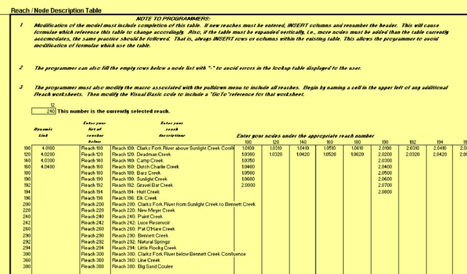 Figure 8-1. Reach/Node Description Table
The Programmer does not need to modify the macros associated with the pull down menu and reach navigation menus at the top of each worksheet. However, the programmer does need to modify the macros associated with the reach maps. A sample of the macro is shown in Figure 8-2. The user simply changes the macro name and reference to match the reaches required. These macros are referenced by the lines in the reach maps.
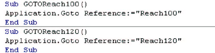
Figure 8-2. Reach Map Navigation Menu
8.3.2 Results Navigator
This portion of the worksheet must be customized to correlate with any future versions of this model. Different river basins will have different compact allocation computations and formats. When incorporated into this model, the Summary Navigator worksheet should be modified to allow the User to .jump. directly to the new tables.
8.3.3 Diagram of the Basin
The model node diagrams are dynamically linked to the Reach/Node worksheets. It is also included as a visual reference for orientation to the basin, helping the user understand locations of nodes and connectivity of reaches. The Wind/Bighorn sub-basin diagrams were created in Excel using autoshapes with the appropriate navigational macros assigned to the reach arrows, node circles, and text descriptions so the user may .jump. directly to the desired Reach/Node worksheet.
8.4 Data Input
8.4.1 Master Node List
This list is referenced throughout the workbook by .lookup. functions. The .lookup. functions primarily associate the name of a node with the node number when it is entered at certain locations. This eases input of information in tables such as the Node Tables, Return Flow Tables, etc. In those tables, the Programmer can simply enter the Node number and the Name is filled in automatically. Therefore, whenever a Node is added to a Reach, it must be inserted in this table.
Because the model frequently uses .lookup. functions, it is highly recommended that the Programmer use Excel.s .INSERT ROWS. command whenever adding information to this or other data tables. When information is added this way, formulas referencing the table automatically update to refer to the newly expanded range. If rows are added to the bottom of a listing, the referenced formula will not .find. the new data.
Due to the method of lookup in the node worksheet by other worksheets, the list should be sorted by increasing node numbers.
8.4.2 Diversion Data
These tables are referenced by several other worksheets in the Wind/Bighorn sub-basin models via .lookup. functions and by direct reference.
It is important to note that ALL nodes are included in this table, even if no diversions occur at that node (e.g. gaging station nodes). This simplifies the spreadsheet logic used in the Node Tables. By including all nodes in this table, the Node Tables are all identical and can generally be copied as many times as are needed without modification (see User and Programmer Notes pertaining to the node/reach worksheets for exceptions to this rule). Therefore, if no diversions occur at a node, simply leave the data columns blank or insert zeros.
Because the model uses .lookup. functions to retrieve data from this table, it is highly recommended that the Programmer use Excel.s .INSERT ROWS. command whenever adding information to this or other data tables. When information is added this way, formulas referencing the table automatically update to refer to the newly expanded range. If rows are added to the bottom of a listing, the referring formula will not .find. the new data. After rows are inserted, the Programmer can copy the formulas in the .Name. column to retrieve gage names automatically. The Programmer can also copy the formulas in the .Reach. column to retrieve the reach number automatically from the .Reach/Node Description Table. on the Navigation worksheet.
8.4.3 Import and Export Data
This table is referenced by several other worksheets in the Wind/Bighorn sub-basin models via .lookup. functions. Any imports or exports must be entered here. No computations are conducted within this worksheet.
It is important to note that ALL nodes are included in this table, even if no imports or exports occur there (e.g. gaging station nodes). This simplifies the spreadsheet logic used in the Node Tables. By including all nodes in this table, the Node Tables are identical and can be copied as many times as needed without modification. Therefore, if no diversions occur at a node, simply leave the data columns blank or insert zeros.
Because the model uses .lookup. functions to retrieve data from this table, it is highly recommended that the Programmer use Excel.s .INSERT ROWS. command whenever adding information to this or other data tables.
8.4.4 Return Flow Data
This table is referenced by several other worksheets in the Wind/Bighorn sub-basin models via .lookup. functions. Return flow data for each node must be entered here. No computations are conducted within this worksheet.
It is important to note that ALL nodes are included in this table, even if no imports or exports occur there (e.g. gaging station nodes). This simplifies the spreadsheet logic used in the Node Tables. By including all nodes in this table, the Node Tables are identical and can be copied as many times as are needed without modification. Therefore, if no diversions occur at a node, simply leave the data columns blank or insert zeros.
Because the model uses .lookup. functions to retrieve data from this table, it is highly recommended that the Programmer use Excel.s .INSERT ROWS. command whenever adding information to this or other data tables.
8.5 Model Computation Worksheets
8.5.1 Return Flow
All nodes where diversions occur must be included in the Return Flows worksheet. The worksheet automatically assigns data to the blocks according to the order shown in the reach table on the Navigation sheet. If nodes are added, the Programmer should use Excel.s .INSERT ROWS. command immediately after the last block to insert the appropriate number of new blocks. Once rows are inserted for new nodes, the Programmer can copy an existing .Node Evaluation. table as many times as needed. When the Programmer changes the Node Number, the Node Name and Total Diversions will update automatically with a .lookup. to the Master Node List and the Diversions Data worksheets, respectively. The Programmer modifies the return flow data used on the worksheets in the return flow data worksheet.
To update the .Irrigation Returns: Node Totals Table., the Programmer must first be certain that all nodes are included in the list of nodes. For simplicity, the Programmer can copy the Node Number column from the Master Node List and paste it here. Then the Programmer can copy the remaining portion of a row including Name, Monthly Summation, and Reach number as many times as needed. The Programmer should be cautioned to verify that the ranges referenced in the monthly summation columns span the entire range of Node Evaluation tables following addition of nodes. The Programmer should also be sure to INSERT new rows within the table when they are needed rather than adding rows to the end of the table.
To update the .Irrigation Returns: Reach Totals Table. the Programmer must enter all reach numbers in the appropriate columns and then copy the formulas in the January through December columns. Verify that the range referenced in the monthly summation cells span the entire range of the .Irrigation Returns: Node Totals Table. after it was modified.
8.5.2 Options Table
Incorporation of an .Irrigation Return Pattern. or .Irrigation Return Lag. relationship which differs from those included in this model can be done by either over-writing one of the existing lines or by inserting a new line within the existing table. If irrigation returns are determined to require longer than six months before returning to the river system, a column may be inserted in the Irrigation Return Lags table. However, it is important to note that the formulas of the Irrigation Returns worksheet will need modification to reflect any additional months.
8.5.3 Basin Gain/Loss
Ungaged Basin Gain/Losses must be computed on a Basin-by-Basin basis in a manner as shown in the .Gain/Loss. worksheet. To do this, the Programmer must reference the appropriate gage data, diversion data (iteration 1: estimated actual; iteration 2: simulated diversions on diversion summary sheet), return flow data (iteration 1: estimated actual; iteration 2: model simulated), and reservoir data; building a budget as shown in the worksheet. Each Basin requires construction of an individual table with that Reach.s specific conditions incorporated. At the bottom of each computation table, the Programmer must enter a Basin Name corresponding to the Basin(s) for which the Gains/Losses will be applied. New Basin Gain/Loss tables may be created by copying another table and entering the new node numbers and basin name.
The Basin Names must then be entered into the Summary Table and the tables will automatically update. The Programmer should verify that the lookup formulas in the Basin Gain Table span the entire Basin Gain/Loss Calculation Iteration One tables. The Basin Loss Table is updated by subtracting the downstream gage data from the total inflow to the most downstream basin node. New Basins should be added to the Summary tables by INSERTING new rows as needed.
Ungaged Reach gains are added to the upstream end of a Reach to make them available to diversions within the Reach. Ungaged Reach losses are subtracted at the downstream end. To facilitate this feature, the Programmer must enter the Reach Name in the Reach Gains line at the upstream node of a reach and the Node Table will automatically update. The Reach Name must also be entered in Ungaged Losses line of the Reach.s downstream node and the Node Table will automatically update.
By incorporating Ungaged Gains and Losses, the spreadsheet model is calibrated to match historic gaging data at each gage node.
8.5.4 Node Tables
Adaptation of the Wind/Bighorn sub-basin models for other river basins will require reconstruction of the Reach/Node worksheets on a node-by-node basis. Because all values in the Node tables are obtained via .lookup. functions, this is a relatively easy task.
The Node Inflow to any Node Table is referenced in one of three ways:
Most nodes will be built using the third method described above. In this case, once the Node Inflow cells have been modified as in the example (i.e., Node 80.06), the Node Table may be copied as many times as needed and the Reach can be constructed in a sequential manner.
The Programmer must enter the Node Number in the cell at the top of each Node Table cell and the worksheet will return the Node Name and all corresponding data from the worksheets referenced.
8.6 Summary Worksheets
8.6.1 Outflow Summary
The .Outflow Calculations: By Node. tables were generated using lookup functions which reference the corresponding Reach worksheets. The values in the .Node. column were entered manually and the lookup tables constructed accordingly. If a reach is inserted, then a new block should be inserted within the list at the appropriate location. Formulas will then need to be modified accordingly for the block and the next downstream block in order for the formulas to work correctly.
The .Outflow Calculations: By Reach. table simply references the downstream limit of each .Outflow Calculations: By Node. table.
8.6.2 Diversions Summary
The .Summary of Diversion Calculations: By Node. tables were generated using lookup functions which reference the corresponding Reach worksheets. The values in the .Node. column were entered manually and the lookup tables constructed accordingly. Formulas will then need to be modified accordingly for the block and the next downstream block in order for the formulas to work correctly.
The .Summary of Diversion Calculations: By Reach. table references the .Summary of Diversion Calculations: By Node. tables using SUMIF functions.
The .Comparison of Model Simulated Diversions vs. Full Supply Diversions (Shortage) and vs. Estimated Actual Diversions (Calibration Check). table looks up Estimated Actual Diversions and Full Supply Diversions for each node from the Estimated Actual Diversions Data and the Full Supply Diversions Data worksheets. It also looks up the Model Simulated Diversions from the .Summary of Diversion Calculations: By Node. tables and computes the shortage and the calibration check.
8.7 Specific Instructions for Adding a Single Node to a Model
The Wind/Bighorn sub-basin models have been constructed such that new nodes, representing a new point of diversion, a reservoir, a streamflow gage, an instream flow segment or any other point at which the user needs to evaluate, can be added. The process for adding a new node is described below. Worksheets need to be modified in the order given here.
8.7.1 General
The workbooks have been provided with the .protection mode. enabled for each worksheet. No password has been used, therefore the user must turn the protection feature off to make changes (Tools/Protection / Unprotect Worksheet).
The user may also find it helpful to turn on the row and column headers and the sheet tabs on each worksheet to be modified (Tools/Options/View).
It is recommended that the user make any modifications to the model in the order that is presented below.
8.7.2 Master List of Nodes Worksheet
There are two ways of modifying the Master List of Nodes:
It is recommended that the user use the second approach so that the list remains in numerical sequence.
8.7.3 The Central Navigation Worksheet
The Reach/Node Description table located to the right of the visible screen must be modified. Go to the column containing the reach that you wish to modify. Type in the node number that you wish to add. If this is not the last node in the reach, it is simplest to retype the subsequent nodes in the rows below rather than inserting a cell.
8.7.4 Gage Data/Inflow Data Worksheet
If the new node to be added represents a gage or an inflow point to the model, the Gage Data/Inflow Data worksheet must be modified. As with the Master List of Nodes, the user can add the new node and relevant data in the next available unused row in the table (as defined by the borders and shading). Alternatively, the user can INSERT a row in the appropriate location to maintain the reach/node sequence, then add the new node and data.
8.7.5 Diversion Data Worksheet
All nodes MUST be included in this table even if no diversion occurs at the node. The user may simply enter the new node and relevant data in the next available unused row in the table (as defined by the borders and shading) or the user can INSERT a row in the appropriate location to maintain the reach/node sequence, then add the new node and data. As a default, there are no unused rows in the table, therefore, the data must be inserted. All four of the diversion worksheets (historical data, full supply data, futures data and the modeled data) must be modified.
8.7.6 Import and Export Data Worksheet
All nodes MUST be included in this table even if no import or export occurs at the node. The user may simply enter the new node and relevant data in the next available unused row in the table (as defined by the borders and shading) or the user can INSERT a row in the appropriate location to maintain the reach/node sequence, then add the new node and data. As a default, there are no unused rows in the table, therefore, the data must be inserted.
8.7.7 Return Flow Data
All nodes MUST be included in this table even if no diversions occur at the node. The user may simply enter the new node and relevant data in the next available unused row in the table (as defined by the borders and shading) or the user can INSERT a row in the appropriate location to maintain the reach/node sequence, then add the new node and data. As a default, there are no unused rows in the table, therefore, the data must be inserted.
The user must then update the .Efficiency Pattern., .Return Pattern., .TO. and .Percent. cells (shaded yellow) to represent conditions associated with the diversions from the new node.
8.7.8 Return Flows Worksheet
All nodes where diversions occur MUST be included in the Return Flows worksheets (both the Estimated Actual Return Flows and the Model Simulated Return Flows must be updated). As a default, all nodes have been included in this list. Select an entire Irrigation Return table and COPY the selected cells. Then, immediately downstream of the last table, select INSERT COPIED CELLS and select SHIFT CELLS DOWN. All data will be updated (note that the new block will contain data for the last node in the model.
To update the .Irrigation Returns: Node Totals Table., the user must first be certain that all nodes are included in the list of nodes. For simplicity, the user can copy the Node Number column from the Master Node List and paste it here. Be sure that the Master Node List does not extend past the yellow shaded area. Then the user can copy the Monthly Summation and Reach number equations as many times as needed. The user should be cautioned to verify that the ranges referenced in the monthly summation columns span the entire range of Node Evaluation tables following addition of nodes.
As currently constructed, the .Irrigation Returns: Reach Totals Table. requires no modification for the simple addition of a node.
8.7.9 Options Table Worksheet
Incorporation of an .Irrigation Return Pattern. or .Irrigation Return Lag. relationship which differs from those included in this model can be done by either over-writing one of the existing lines or by inserting a new line within the existing table. If irrigation returns are determined to require longer than six months before returning to the river system, a column may be inserted in the Irrigation Return Lags table. However, it is important to note that the formulas of the Irrigation Returns worksheet will need modification to reflect any additional months.
8.7.10 Evaporative Losses Worksheet
If the new node is a storage node, COPY the rows containing the .Mean Monthly Evaporation (inches)., .Historical End-of-Month Contents (acre-feet). and .Surface Area (acres). tables and insert the rows above the .Mean Monthly Evaporation (acre-feet). table. Update the node number and the node name will automatically update. Enter gross evaporation and precipitation for the new node. Enter the historical end-of-month contents for the reservoir. If the gross evaporation and precipitation are the same for the new node as for any existing nodes, only the .Historical End-of-Month Contents. and .Surface Area. tables need to be copied (or rows inserted in the existing tables).
Select and COPY the rows containing the existing area-capacity table, then paste the rows below the existing table. Update the node number and area-capacity information.
The reservoir surface area is calculated by looking up historical end-of-month content and interpolating the surface area from the area-capacity table. The .vlookup. portion of the equation must be updated to correspond to the new area-capacity table.
Enter a new node number and the equation to calculate the mean monthly evaporation within the .Mean Monthly Evaporation (acre-feet). table. If there is no room available in the table, INSERT a row within the table and add the necessary information.
8.7.11 Basin Gain/Loss Worksheet
Determine the ungaged basin gain/loss table that the new node is within. Locate the corresponding table in the Basin Gain/Loss Worksheet. Select the row in the diversion portion of the table either above or below where the new node needs to be inserted. COPY the selected cells, then INSERT COPIED CELLS in the appropriate location. Update the node number in the yellow shaded cell. The node name and diversions associated with the new node will automatically update. Repeat these steps in the return flow portion of the table. This should be done to both the Iteration One and the Iteration Two worksheets.
8.7.12 Reach/Node Worksheet
Select the rows containing an entire Node table. COPY the selected rows, then move to the new location in the workbook and select INSERT COPIED CELLS. Update the node number in the yellow shaded cell. The node name, diversions, irrigation returns, ungaged gains/losses and import/exports will automatically update if all the above steps have been completed.
The Node Inflow to any Node Table references one of three sources:
Most nodes will be built using the third method described above.
If the Reach/Node table represents a reservoir, the user will need to manually update the cells shaded yellow.
As a precautionary measure, it is best to check the Node Inflow in the Reach/Node table below where the new node has been inserted to ensure that the appropriate cells are referenced.
Section 9 - References
Anderson Consulting Engineers. 2000. .Bear River Basin Plan Task 3B. Surface Water Spreadsheet Model Development.. Technical Memorandum, Fort Collins, Colorado. September 18.
Boyle Engineering Corporation. 2001. .Green River Basin Plan Surface Water Data Synthesis and Spreadsheet Model Development.. Technical Memorandum, Denver, Colorado. January 2.
BRS, Inc. 2002. .Wind/Bighorn River Basin Plan Water Supply and Demand in the Wind/Big Horn Basin.. Technical Memorandum, Riverton, Wyoming.
BRS, Inc. 2003. .Wind/Bighorn River Basin Plan Irrigation Diversion Operation and Description.. Technical Memorandum, Riverton, Wyoming.
HKM Engineering Inc. 2001. .Powder-Tongue River Basin Plan Spreadsheet Model Development and Calibration, Task 3B.. Technical Memorandum. December.
Lidstone and Associates (LA). 2002. .Wind/Bighorn River Basin Plan Water User From Storage.. Technical Memorandum.
Lidstone and Associates (LA). 2002. .Wind/Bighorn River Basin Plan Municipal Basin Water Use Profile.. Technical Memorandum.
MWH. 2002. .Wind/Bighorn River Basin Plan Task 3A/3B - Surface Water Hydrology.. Technical Memorandum. Denver, Colorado.
MWH. 2003a. .Wind/Bighorn River Basin Plan Task 2A . Agricultural Water Use and Diversion Requirements.. Technical Memorandum. Denver, Colorado.
MWH. 2003b. .Wind/Bighorn River Basin Plan Task 3D . Available Surface Water Determination.. Denver, Colorado.