Wyoming State Water Plan
Wyoming State Water Plan
Wyoming Water Development Office
6920 Yellowtail Rd
Cheyenne, WY 82002
Phone: 307-777-7626

Wyoming Water Development Office
6920 Yellowtail Rd
Cheyenne, WY 82002
Phone: 307-777-7626
CHAPTER 3 SURFACE AND GROUNDWATER AVAILABILITY
3.1 . Surface Water Hydrology
3.1.1 . Introduction
An important part of the river basin planning process is to estimate water availability within the river basins for future development and use, this includes both surface water and ground water. The availability of surface water was determined through the construction and use of a spreadsheet simulation model that calculates water availability based on the physical amount of streamflow less historical diversions, compact requirements and minimum flows. The availability of ground water was primarily performed based on a review of existing information throughout the study area.
The Guidelines for Development of Basin Plans (WWDC, 2001) recommends that for the purposes of the river basin planning process, a hydrologic analysis be conducted for three 12-month periods using average dry-year conditions, average average-year conditions and average wet-year conditions. Therefore, each hydrologic region in the model has three associated spreadsheet models representing those three hydrologic conditions. The gaged flows used in the spreadsheet model are developed by averaging recorded monthly streamflows for groups of years falling into those three hydrologic categories during a consistent period of record.
A study area map containing major sub-basins and locations of key gages and index gages (as described later in the text) is presented in Figure 3.1-1. The study area includes the Missouri River Basins located in northwestern Wyoming, including the portions of the Madison River Basin, Gallatin River Basin, Yellowstone River Basin and Wind/Bighorn River Basin located within the State of Wyoming. Table 3.1-1 shows the USGS Hydrologic Unit classifications, which are included in the planning area and the model in which each sub-basin is included. All of the river basins are tributary to the Yellowstone River in southern Montana, which is subsequently tributary to the Missouri River in western North Dakota.
For purposes of the discussion herein, the Study Area was divided into five basins: the Madison/Gallatin River Basin, the Yellowstone River Basin, the Wind River Basin and the Bighorn River Basin. The Madison River and Gallatin River are not hydrologically connected, however, they were grouped together because the models are very small. The Wind and Bighorn Rivers are actually the same river, changing names at the .Wedding of the Water. near Thermopolis. The river is called the Wind River south of the Owl Creek Mountains while it is called the Bighorn River north of the Owl Creek Mountains. The river was separated because of the clear basin distinctions that occur through the Owl Creek Mountains. There are no hydrologic connections, other than the river itself, across the mountain chain.
Table 3.1-1 USGS Hydrologic Units and Associated Models Included in Study Area
| Hydrologic Unit Code | USGS Hydrologic Unit Name | Area (acres) | Study Basin | Study Sub-Basin | Model |
| 10020007 | Madison | 1,638,991 | Madison/Gallatin | Madison/Gallatin | Madison/Gallatin |
| 10020008 | Gallatin | 1,162,356 | Madison/Gallatin | Madison/Gallatin | Madison/Gallatin |
| 10070001 | Yellowstone Headwaters | 1,654,127 | Yellowstone | Yellowstone | Yellowstone |
| 10070002 | Upper Yellowstone | 1,897,992 | Yellowstone | Yellowstone | Yellowstone |
| 10070006 | Clarks Fork Yellowstone | 1,784,937 | Clarks Fork | Clarks Fork | Clarks Fork |
| 10080001 | Upper Wind | 1,628,472 | Wind | Upper Wind | Upper Wind |
| 10080002 | Little Wind | 708,641 | Wind | Little Wind | Little Wind |
| 10080003 | Popo Agie | 511,611 | Wind | Not Included(1) | Not Included(1) |
| 10080004 | Muskrat | 466,187 | Wind | Lower Wind | Lower Wind |
| 10080005 | Lower Wind | 1,084,233 | Wind | Lower Wind | Lower Wind |
| 10080006 | Badwater | 538,167 | Wind | Badwater | Lower Wind |
| 10080007 | Upper Bighorn | 2,217,263 | Bighorn | Upper Bighorn | Upper Bighorn/Owl Creek |
| 10080008 | Nowood | 1,282,397 | Bighorn | Nowood | Nowood |
| 10080009 | Greybull | 733,218 | Bighorn | Greybull | Greybull |
| 10080010 | Bighorn Lake | 1,150,802 | Bighorn | Bighorn Lake | Lower Bighorn |
| 10080011 | Dry | 281,821 | Bighorn | Bighorn Lake/Greybull | Lower Bighorn |
| 10080012 | North Fork Shoshone | 545,062 | Bighorn | Shoshone | Shoshone |
| 10080013 | South Fork Shoshone | 417,701 | Bighorn | Shoshone | Shoshone |
| 10080014 | Shoshone | 954,605 | Bighorn | Shoshone | Shoshone |
Notes:
(1)The Popo Agie River Basin is modeled in the Popo Agie River Watershed study. This model contains an inflow node for the Popo Agie River that incorporates these results.
3.1.2 . Historical Streamflow Records
The basin spreadsheet models utilize historical data to simulate river operations on a monthly basis during average dry, average and wet years. Therefore, data collection and reduction to useable formats within the model was the first task in the modeling effort.
Streamflow data were available for hundreds of locations throughout the study area for various periods of record. Streamflow gages are primarily operated and maintained by the U.S. Geological Survey (USGS), while the State Engineers Office (SEO) has historically operated miscellaneous gages in the Wind/Bighorn River Basin (WBHB) for brief periods to assist in water delivery and accounting. USGS data available from both the Wyoming Water Resources Data System (WRDS) and the USGS National Water Information System (NWIS) on the Internet (USGS, 2002). USGS data used in this model was researched using WRDS, then downloaded from the Internet to facilitate incorporation into existing data reduction spreadsheets.
Separate spreadsheets for each hydrologic unit were developed to store streamflow data. Typically, the base reporting level for the USGS is average daily streamflow in cubic feet per second (cfs). Therefore, in order to have available the most detailed records in the database, the average daily streamflow was downloaded from the Internet and stored in the spreadsheet. Then, the spreadsheet was used to reduce daily data into total monthly flow and total annual flow in acre-feet for each month and year that data were available.
3.1.3 . Study Period Selection
Because historical data is not available for all gages since the inception of data collection, and to make the model less expansive and easier to use, a representative study period was selected from the data set. The study period is intended to be representative of the overall long-term gage records and hydrologic conditions. To be consistent within the study period, overall patterns of basin inflows, diversions and storage must remain constant through the study period. Therefore, study periods were selected to minimize the impacts of major reservoirs or diversion projects within the period of record. This required examination of reservoir and diversion construction records. Streamflow statistics within each study period were checked against long-term statistics at gages with long-term records to ensure that the data were representative of the long-term period.
The following events were considered in selection of a model study period. Note that this list of events focuses primarily on significant events during the past 50 years that could have had significant impacts on streamflow.
As shown, there is no time period that would completely eliminate impacts of new projects within the period-of-record. However, several events occurred between the 1950.s and early 1970.s, which would have had a substantial impact on river flows. In addition to the major projects shown above, use of more modern irrigation practices such as gated pipe and sprinklers also increased significantly during the early 1970.s. Therefore, for purposes of this study, a study period of 1973-2001 was chosen. This period is especially beneficial in that for most of the basins, both the driest and wettest years on record are contained in the study period. A brief summary of the selected study period as compared with overall streamflow records for each major sub-basin is presented in the following paragraphs.
A statistical summary of the period-of-record and the study period for the Clarks Fork of the Yellowstone River near Belfry is presented in Table 3.1-2. As shown, the average flow during the study period is approximately 2.0% less than the long-term average. In addition, the hydrologic year averages for the study period are all slightly less than the long-term average, which results in the model being slightly conservative towards water supply in general.
Table 3.1-2 Statistical Summary for Clarks Fork Yellowstone River near Belfry (06207500)
| Statistic | Period-of-Record | Study Period | Difference |
| 1922 . 2001 | 1973-2001 | ||
| Mean | 678,048 | 664,349 | -2.0% |
| Standard Deviation | 156,308 | 170,919 | 9.3% |
| Average . Dry Years | 482,266 | 430,150 | -10.8% |
| Average . Average Years | 659,734 | 658,300 | -0.2% |
| Average . Wet Years | 928,773 | 915,688 | -1.4% |
| Maximum | 1,075,109 | 1,075,109 | 0.0% |
| Minimum | 395,919 | 395,919 | 0.0% |
A statistical summary of the period-of-record and the study period for the Little Wind River near Riverton is presented in Table 3.1-3. As shown, the average flow during the study period is approximately 2.2 percent less than the long-term average. For the hydrologic year classification, the dry and average years are slightly drier than the long-term average, while the wet years are slightly wetter than the long-term average, which will generally make the model slightly conservative regarding water supply. However, if excess water were used to fill a reservoir for carryover storage, the model may show that there is slightly more water available to fill the reservoir during wet years than what has been available during the long-term average.
Table 3.1-3 Statistical Summary for Little Wind River Near Riverton (06235500)
| Statistic | Period-of-Record | Study Period | Difference |
| 1942 . 2001 | 1973-2001 | ||
| Mean | 417,778 | 408,775 | -2.2% |
| Standard Deviation | 151,116 | 169,197 | 12.0% |
| Average . Dry Years | 212,305 | 199,337 | -6.1% |
| Average . Average Years | 415,338 | 396,907 | -4.4% |
| Average . Wet Years | 630,568 | 651,841 | 3.4% |
| Maximum | 739,201 | 739,201 | 0.0% |
| Minimum | 126,379 | 126,379 | 0.0% |
A statistical summary of the period-of-record and the study period for the Shell Creek near Shell is presented in Table 3.1-4. As shown, the average flow during the study period is approximately 0.2 percent less than the long-term average. For the hydrologic year classification, the dry years are significantly drier than the long-term average, the wet years are slightly drier and the average years slightly wetter than the long-term averages. With the drier years, the dry years will generally make the model slightly conservative regarding water supply.
Table 3.1-4 Statistical Summary for Shell Creek Near Shell (06278500)
| Statistic | Period-of-Record | Study Period | Difference |
| 1942 . 2001 | 1973-2001 | ||
| Mean | 70,879 | 70,758 | -0.2% |
| Standard Deviation | 14,258 | 13,904 | -2.5% |
| Average . Dry Years | 64,545 | 50,416 | -21.9% |
| Average . Average Years | 71,812 | 72,046 | 0.3% |
| Average . Wet Years | 89,192 | 87,452 | -2.0% |
| Maximum | 98,394 | 98,394 | 0.0% |
| Minimum | 37,374 | 37,374 | 0.0% |
3.1.4 . Data Filling and Extension
Many of the gages used in the model have an incomplete record or have periods within the record where data is missing. Therefore, in order for the gage data to be used in the model, the period-of-record for the gage requires either extension or filling. For purposes of this analysis, the same methodologies were used for both filling of gage records and extension of gage records. In addition, the gage records were only filled or extended for those periods in the selected study period (1973-2001).
Many methods can be used for filling gage records. The most common and easiest to use method is regression of measured streamflow at the dependent gage (the gage where data filling is required) to measured streamflow at the independent gage (the gage where data exists for the missing period). Once this mathematical relationship is established, measured data from the independent gage can be used to estimate the streamflow for the dependent gage. Typical regression relationships can be based on linear, polynomial, power or logarithmic relationships. For this study most of the strongest relationships were found to be either linear or polynomial in nature. The measure of the degree to which the two gages correlate is typically called the correlation coefficient (or r2 value). A correlation coefficient of 1.0 indicates perfect correlation. Therefore, those relationships with correlation coefficients closer to 1.0 have good correlation. Typically, in streamflow data filling and extension, correlation coefficients greater than approximately 0.7 are desired. When correlation coefficients are less than this value, then relationships are considered weak, and attempts to find gages with better relationships are made. Correlations were developed between monthly streamflows.
For a majority of the gages, monthly regressions with nearby streamflow gages yielded acceptable correlations to fill the records. However, for the gages where correlations were weak, attempts were made to find other relationships to fill the streamflow values. First, regressions with precipitation data were attempted. This regression is typically more valid where snowmelt is not a significant component of streamflow, which limits its use in the study area. Another methodology that can be used is correlation between annual streamflows, then distribution of annual streamflow to monthly streamflow using historical distributions. If the annual streamflow regression correlation was weaker than the original monthly streamflow correlation, then the monthly regression was used. Finally, the streamflow record can be filled using regional equations based upon basin characteristics. However, this methodology is only used in rare occasions when the correlation coefficient is extremely weak. This methodology was not used for any of the streamflow gaging stations. Overall, approximately 88 percent of the gages filled had correlation coefficients greater than 0.7, while all but one station had correlation coefficients greater than 0.5.
3.1.5 . Ungaged Headwater Site Data Estimation
In order for the model to accurately simulate streamflow and diversions for the entire WBHB, an estimation of streamflow above all diversions is required. However, in many parts of the WBHB, there are no streamflow gaging stations above the most upstream diversion on the stream. Therefore, streamflow upstream of the diversion must be estimated. Two methods are available to make these estimations:
For most locations, the regional equation methodology was used to estimate streamflow for ungaged headwater sites. However, in areas where this methodology yielded implausible results, such as the streamflow being less than the actual measured diversion, or the streamflow being greater than the next downstream gage adjusted for inflows and diversions, then the estimated headwater flows were adjusted based on the available data. More detailed explanations are found in the detailed model description chapters.
For the study area, two sources of regional regression equations are available for estimating natural flows. The USGS (Rankl, 1994) has published monthly regression equations for the Wind River Basin based upon several physical basin characteristics, including drainage area, mean basin elevation, basin slope, maximum basin relief and mean annual precipitation. Discharges are given for the 10, 50, 70 and 90 percent exceedance levels (Q10, Q50, Q70 and Q90). For purposes of this report, Q10 was used for wet years, Q50 was used for average years and Q90 was used for dry years. Monthly regional regression equations for the entire State of Wyoming were developed by Miselis (1999). Equations were developed for the Wind, Bighorn and Absoraka ranges within the study area and are a function of drainage area and precipitation. The USGS study was used for the Wind River Basin (because the study was more specific to the WBHB) while the Miselis data were used for the other two areas. Physical data were estimated using various Geological Information Survey (GIS) coverages and techniques.
3.1.6 . Hydrologic Year Classification
Once the study period was selected, the monthly data were further reduced into average data for dry, average and wet hydrologic year classifications. To determine which years within the period-of-record fall into which hydrologic year classifications, index gages were selected within each of the hydrologic units. These gages were selected based upon their period-of-record and their lack of influence by diversions and return flows. Then, the hydrologic classification for the index gage was applied to the remaining gages within its influence area. The hydrologic classifications for the WBHB plan are consistent with the hydrologic classifications for the other river basin plans and with the guidelines. A summary of the classification methodology is shown in Table 3.1-5, while a summary of the hydrologic year classification for each index gage is shown in Table 3.1-6. Locations of the index gages are presented in Figure 3.1-1.
Table 3.1-5 Hydrologic Classification Methodology
| Dry | Average | Wet | |
| Percent of Years | Driest 20 percent | Middle 60 percent | Wettest 20 percent |
| Number of Years in 29-year Study Period | 6 | 17 | 6 |
Table 3.1-6. Summary of Hydrologic Classifications for Study Area
| Basin | USGS Gage No | Gage ID | 1970 | 1980 | 1990 | 2000 | |||||||||||||||||||||||||
| 3 | 4 | 5 | 6 | 7 | 8 | 9 | 0 | 1 | 2 | 3 | 4 | 5 | 6 | 7 | 8 | 9 | 0 | 1 | 2 | 3 | 4 | 5 | 6 | 7 | 8 | 9 | 0 | 1 | |||
| Mad./Gal., Yell., Ck. Fk. | 06037500 | Madison Near West Yellowstone | |||||||||||||||||||||||||||||
| 06191500 | Yellowstone At Corwin Springs | ||||||||||||||||||||||||||||||
| 06205500 | Clarks Fk Ab Squaw Ck | ||||||||||||||||||||||||||||||
| Wind | 06222700 | Crow C Nr Tipperary Wyo | |||||||||||||||||||||||||||||
| 06224000 | Bull Lake Creek Above Bull Lake | ||||||||||||||||||||||||||||||
| 06228350 | SF Little Wind Ab Washakie Res | ||||||||||||||||||||||||||||||
| Bighorn | 06260000 | South Fork Owl Ck Near Anchor | |||||||||||||||||||||||||||||
| 06270000 | Nowood River Near Tensleep | ||||||||||||||||||||||||||||||
| 06275000 | Wood River At Sunshine | ||||||||||||||||||||||||||||||
| 06278500 | Shell Creek Near Shell | ||||||||||||||||||||||||||||||
| 06280300 | SF Shoshone River Near Valley | ||||||||||||||||||||||||||||||
| Notes: | |||
| (1) | Hydrologic Year Classification | - Wet Year (Wettest 20 percent of years) | |
| - Average (Middle 60 percent of years) | |||
| - Dry Year (Driest 20 percent of years) | |||
Both the Madison River near West Yellowstone gage and the Gallatin River gage contain adequate data to classify hydrologic years. However, since the primary gages that need to be classified in the model are Madison River tributaries, the Madison River near West Yellowstone gage (06037500) was selected for the analysis.
There are three gages within the Yellowstone model that would be adequate for hydrological classification: the Yellowstone River at the Yellowstone Lake Outlet (06186500), Gardner River near Mammoth (06190500) and the Yellowstone River at Corwin Springs (06191500). The first two gages, respectively, have short periods where data would need to be filled. In addition, the annual flow variation at the Yellowstone Lake Outlet gage is small and may not provide a good measure of hydrologic variability throughout the entire WBHB. Therefore, the Corwin Springs gage was selected as the index gage for the entire WBHB.
Although the Clarks Fork near Belfry gage contains continuous data through the period-of-record, the gage is located downstream of agricultural diversions. These diversions have an influence on the relative flow at the gage making it unsuitable for use as an index gage in the hydrologic year classification. Two other gages within the WBHB are located upstream of diversions making them more suitable for use as the index gage: the Clarks Fork Yellowstone River above Squaw Creek and Sunlight Creek near Painter. Neither of these gages have any data in the study period. However, since the correlation coefficients used to fill the data were very strong, the filled data should be representative of actual flows at the gage, allowing either to be used as an index gage. Because the Clarks Fork above Squaw Creek gage is on the mainstem and contains a larger portion of flow in the WBHB, it was selected as an index gage.
Several gages within the Wind River Basin contain adequate data to serve as index gages for development of hydrologic year classifications. As with previous index gage selection, gages that are not significantly influenced by diversions, storage or return flows are the most desirable gages. For the Wind River Basin, to account for differences in hydrology between sub-basins and location of gages, separate gages were selected for sites along the Wind River range in the Wind River sub-basin and Little Wind River sub-basin, and those located along the Owl Creek range. For purposes of this analysis, the following gages were selected as index gages: Bull Lake Creek above Bull Lake (06224000), South Fork Little Wind River above Washakie Reservoir (06228350) and Crow Creek near Tipperary (06222700).
Only a few gages within the Bighorn Basin contain adequate data to serve as index gages for development of hydrologic year classifications. As with previous index gage selection, gages that are not significantly influenced by diversions, storage or return flows are the most desirable gages. In the Bighorn Basin, separate gages were selected for sites along the Owl Creek Range in the Upper Bighorn Basin and Nowood River Basins, the Bighorn range in the Nowood River Basin, and Bighorn Lake River Basin, and the Absaroka range in the Greybull and Shoshone River Basins. For purposes of this analysis, the following gages were selected as index gages: the South Fork of Owl Creek near Anchor (06260000), Nowood River near Tensleep (06270000), Wood River at Sunshine (06275000), Shell Creek near Shell (06278500) and the South Fork Shoshone River near Valley (06280300).
3.2 . Spreadsheet Model Development and Calibration
3.2.1 . Introduction
The Guidelines for Development of Basin Plans (WWDC, 2001) and WWDC required that the river basin planning models be consistent with the other models that have already been developed. The original spreadsheet model was developed by Anderson Consulting Engineers for the Bear River Basin, which was the initial pilot study for the river basin planning process. That model was utilized as a base model for the Green River Basin Plan by Boyle Engineering, which was subsequently used by HKM as a base model for the Powder-Tongue and Northeast River Basin Plans. Improvements in the model were made upon each successive iteration of the model, including improvements in data entry, calculation methodologies and the Graphical User Interface (GUI). It should be recognized that the models are quite general in nature and although they provide a reasonable indication of water availability on any given stream, caution should be exercised in drawing conclusions from the results about individual diversions or water uses.
USGS Hydrologic Unit classifications and their associated models were previously shown in Table 3.1-1. As shown, the study area has been divided into 12 models. The models generally follow the same areas as the study sub-basins, with the following exceptions:
The models are intended to simulate existing river operations for dry, average and wet year hydrologic periods. In general, existing operations are reflected in the historical operations within the study period. In a few instances where existing conditions are different than either a portion or all of the historical conditions, special provisions in the data input and modeling calibration were required and are documented within the calibration section of Technical Memorandum, Chapter 3, Tab 15 Spreadsheet Model Development and Calibration.
The primary data required for the spreadsheet models are streamflow, actual (or estimated actual) diversions, full supply diversions, irrigation returns and reservoir operations. For each of these, the data within the study period was reduced into dry, average and wet year data. The reduction of streamflow data, including the calculation of natural flow data for those tributaries that do not contain diversions, is described in the Surface Water Hydrology Technical Memorandum. Development and reduction of actual diversion data is discussed in the Technical Memorandum Irrigation Diversion Operation and Description, Task 2A Technical Memorandum Agricultural Water Use and Diversion Requirements., while the estimation of actual diversion for those diversions without actual measurements is discussed later in this report.
The model is run on a monthly timestep for the given calendar year of the hydrologic condition (dry, average, and wet). Starting reservoir levels are the same as the historical end-of-month contents on the last day for that hydrologic condition (i.e., the dry year model starting contents in January is the historical dry year end-of-month contents in December).
The basic model calculation procedure is shown in Figure 3.2-1. Natural flows for each main channel and tributary are either taken from gage data (preferred but not normally available) or estimated using the regional regression techniques as describe in the Task 3A/3B Technical Memorandum Surface Water Hydrology. Then, the incremental gains and losses are calculated for each reach. This is performed by locating the first downstream gaged node and constructing a .basin. containing all of the known upstream inflows, diversions and reservoir operations. The basins often contain many tributaries to the gaged node. Once the ungaged gains and losses are calculated, they are distributed to each reach within the basin by pro-rating the gains and losses based upon the reach.s contribution to the gage flow. Ungaged gains are applied at the top of the reach to allow for diversion, while the ungaged losses are applied to the bottom of the basin to allow diversion of computed inflows.
Once the ungaged gains and losses are calculated, a mass balance (or water budget) is computed at each node. At nodes other than storage nodes, the amount of flow available to the next downstream node is calculated as the difference between known inflows, such as tributary inflows, return flows, basin gains and imports, and outflows, such as diversions, basin losses and exports. At storage nodes, the losses due to evaporation and the gains/losses due to change in storage are included in the calculations. Diversions are limited to the lesser of the full supply diversion and the physical streamflow. The mass balance is performed from upstream to downstream for each node in the reach, and for each reach in the model.
Model output includes the following:
The limitations of the model should be noted:
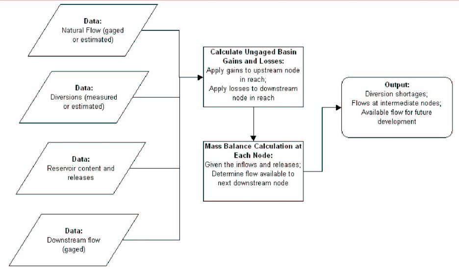
Figure 3.2-1 Generalized Model Flowchart
3.2.2 . Model Development
As with the previous river basin plans, the models for the Wind/Bighorn River Basin plans were developed using Microsoft? Excel 97. All computations within the workbooks are performed using formulas written in the cells of the workbooks. The workbooks also contain macros that are used only for navigation between the various worksheets in the workbooks. The model calculations are completely automated so that when data is changed in any cell, the entire model is updated. The one exception is when data is shared between models. The procedures for sharing data between models are discussed in more detail later in this document.
As requested by the WWDC, the models were developed for the novice Excel user. Basic proficiency in spreadsheet usage is required to view results and to make minor changes to input data and variables. However, to input additional nodes or reaches in the model, a more advanced level of proficiency is required. Interactive buttons have been placed throughout the spreadsheets to allow for easier navigation between the spreadsheets. All .tabs. and .row-column headers. within the model have been activated as it was found that for most users, this information is useful to view. Also, due to the size and calculation time of the models, .manual calculation. has been selected as the calculation procedure. In this mode, model calculations are not performed until the users hits the .F9. key on the keyboard. Extreme caution should be exercised by those wishing to make changes to the model construction.
3.2.3 . Model Schematics
The physical structure of each model is represented in the river basin schematics and the reach schematics. Separate schematics have been developed for each model. The development of these schematics is discussed in the following paragraphs.
The river basin schematics are detailed link-node representations of the river basins. The schematics include nodes representing streamflow gages, natural flow nodes, diversion nodes, lumped diversion nodes, points of confluence and specific points of return flows if not already represented by a node. The nodes are connected by a series of links that represent the actual flow of water (normally in a stream) between the nodes. It should be noted that for visual clarity, the schematics are connected by straight links and are not to scale. Normally, the general flow direction through the schematic mirrors the actual flow direction, with north pointing towards the top of the schematic.
The reach schematics are simplified versions of the river basin schematics that are developed on a .reach. basis. Reaches are a group of nodes that represent an entire tributary or a portion of the main river. As discussed in later sections, the model calculations and water availability are generally performed and reported on a reach basis. The reach schematics are also used for navigational purposes within the model GUI. Reach schmatics for each model are presented in Figures 3.2-2 through 3.2-13.
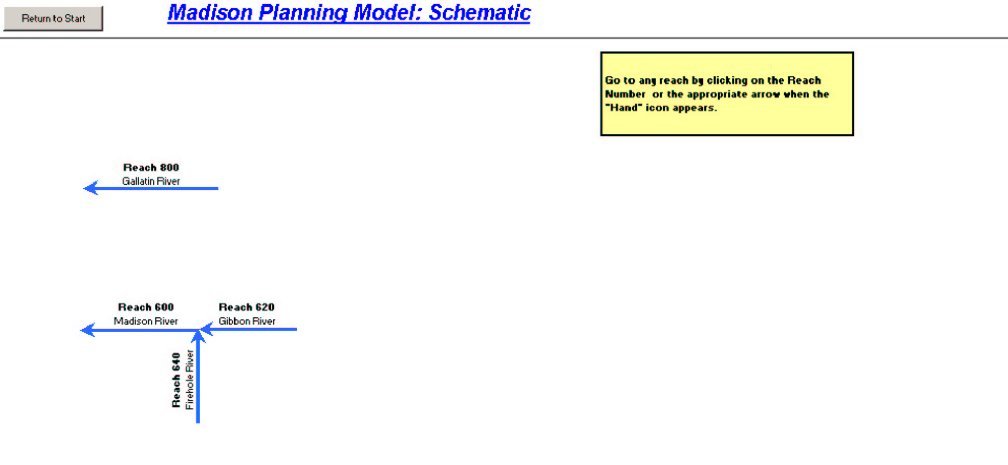
Figure 3.2-2. Reach Schematic - Madison/Gallatin Model
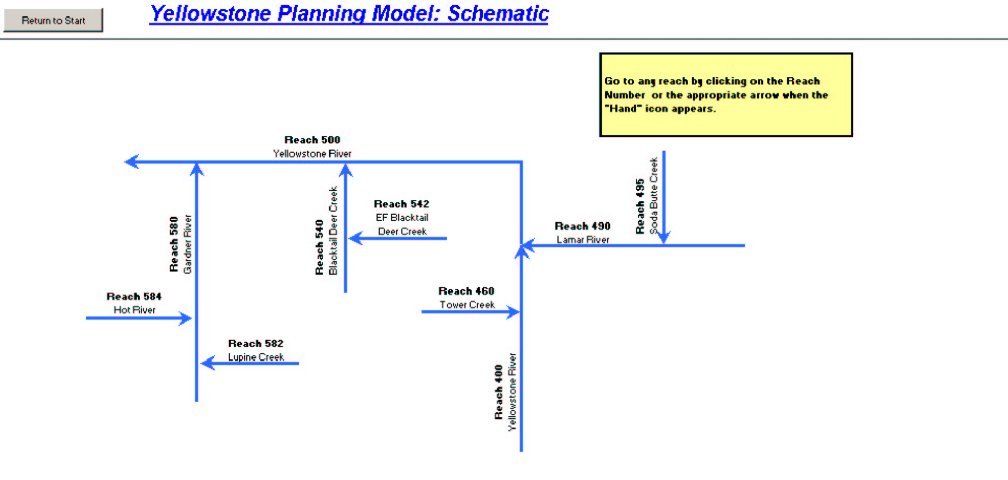
Figure 3.2-3. Reach Schematic - Yellowstone Model
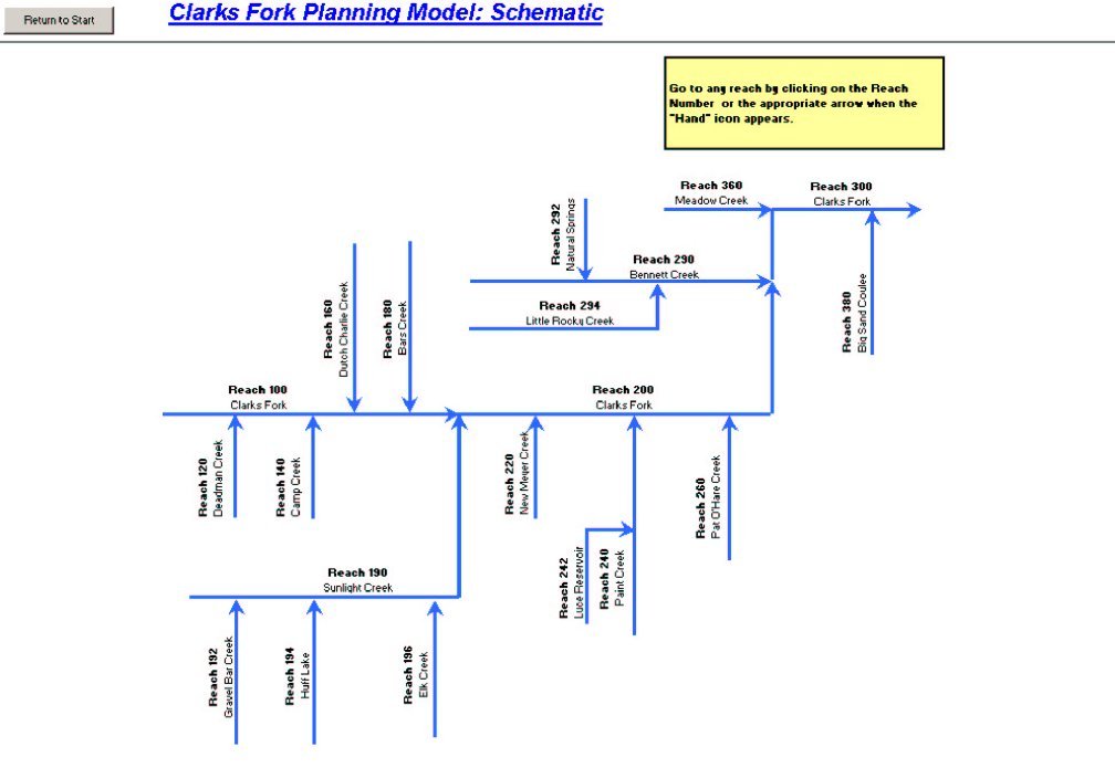
Figure 3.2-4. Reach Schematic . Clarks Fork Model
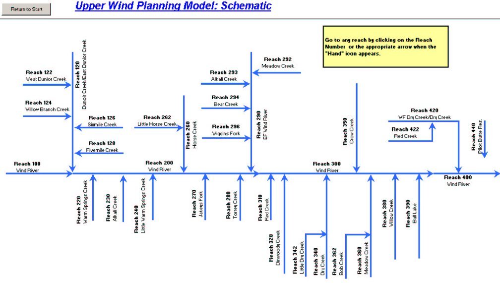
Figure 3.2-5. Reach Schematic . Upper Wind Model
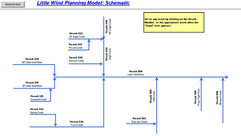
Figure 3.2-6. Reach Schematic . Little Wind Model
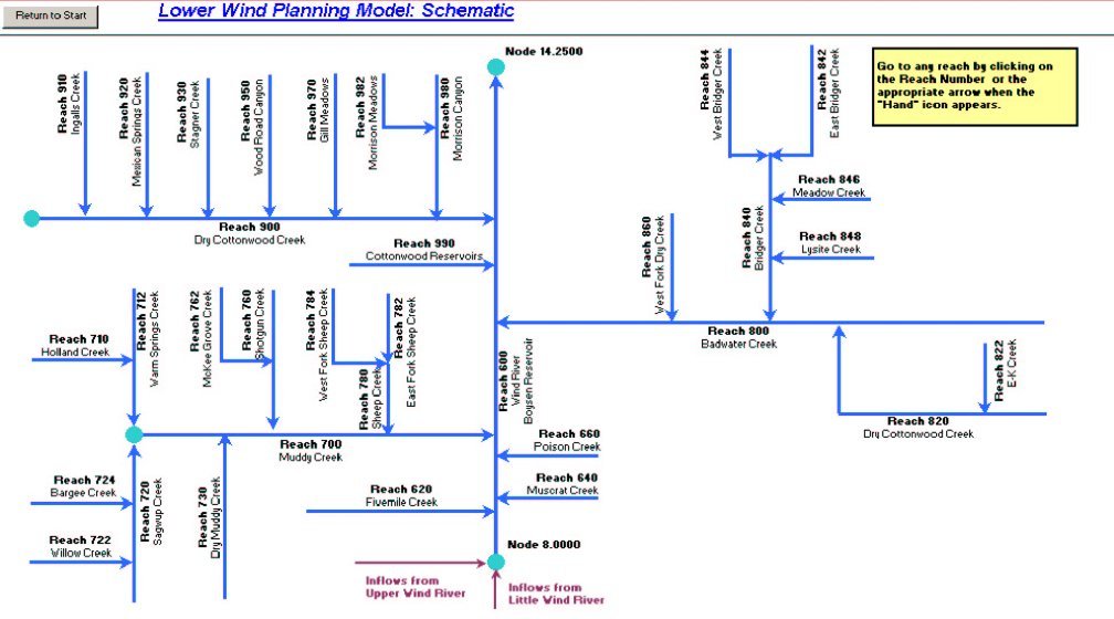
Figure 3.2-7. Reach Schematic . Lower Wind Model
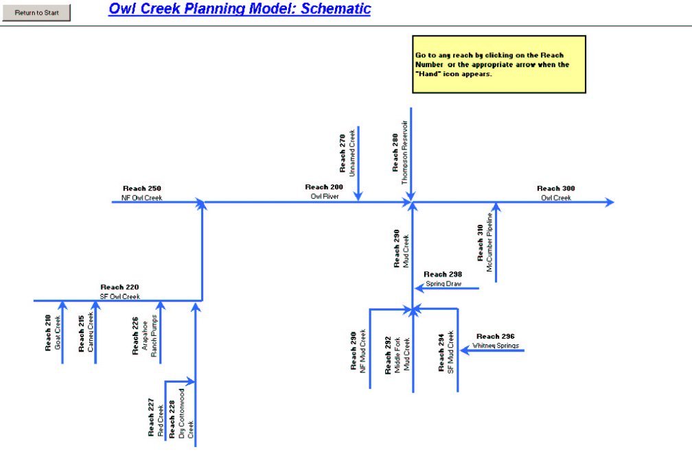
Figure 3.2-8. Reach Schematic . Owl Creek Model
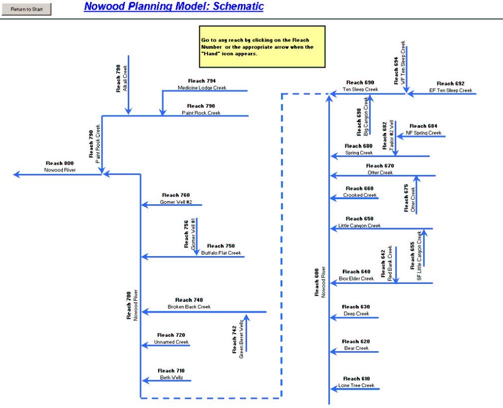
Figure 3.2-9. Reach Schematic . Nowood Model
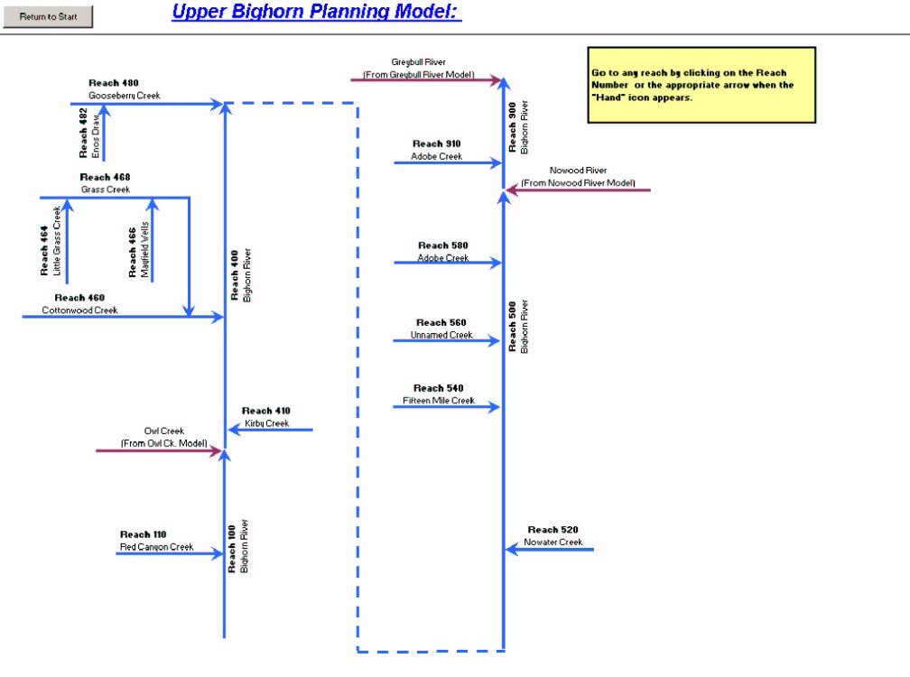
Figure 3.2-10. Reach Schematic . Upper Bighorn Model
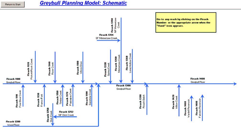
Figure 3.2-11. Reach Schematic - Greybull Model
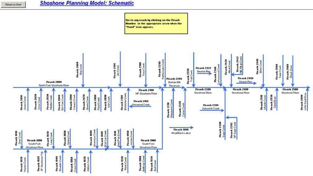
Figure 3.2-12. Reach Schematic - Shoshone Model
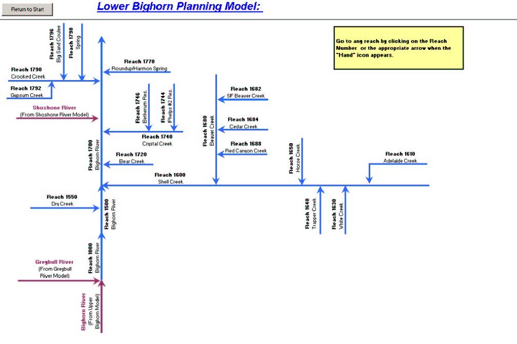
Figure 3.2-13. Reach Schematic . Lower Bighorn Model
3.2.4 . Differences from Previous River Basin Planning Models
As previously indicated, in general, the WBHB planning models are consistent with those developed for previous basins. However, some improvements to the previous models were incorporated to fit the needs of the Wind/Bighorn River Basin plan. The primary difference is that previous models ran the calibration and simulation modes simultaneously. However, in the Wind/Bighorn River Basin Plan, historical diversions were significantly different than full supply diversions. Therefore, calibration was not possible because the model was attempting to divert a full supply diversion, but calibrating to historical streamflows. Therefore, the following additions were made to the model.
The model can be run in three different modes: Calibration (or historical), Full Supply diversions, and Futures diversions. The run mode is selected using buttons on the navigation worksheet.
Because the model can be run in full supply or futures diversion modes, a slightly different calculation methodology was used in the Wind/Bighorn models than in previous models. In previous models, reach losses at the ends of the reaches are calculated based on the downstream gage, so that the simulated gage always matches the calculated gage flow (the ungaged loss calculated in the gain/loss calculations was not used). However, in the Wind/Bighorn models, the streamflows are fully simulated, meaning that the reach loss calculated in the gain/loss calculations is used in the reach calculations. The model is then calibrated using gaged flow versus simulated flow.
3.3 . Available Surface Water Determination
3.3.1 . Introduction
The models are intended as a tool for identifying regional demand shortages and the opportunity for additional water development given major hydrologic and institutional constraints. Per the definition of the calibration mode, the model does not show any shortages at diversions when run in this mode, and thus, no results from this run are presented as part of the results. The results presented herein are for the .Fully Supply for Existing Irrigated Lands. and the .Full Supply for Existing Irrigated Lands and Futures Projects. modes.
3.3.2 . Diversion Shortages
An important result of the WBHB planning models is the calculation of diversion shortages. The model construction allows calculation of shortages at each node in the model. However, it must be realized that the model does not explicitly account for water rights, storage ownership rights or other delivery constraints within the delivery system. Any of the diversions within the WBHB can experience shortages from time-to-time. For instance, in 2001 and 2002, which were drier years than the dry-year used in the modeling hydrology, nearly all diversions within the basins experienced shortages of one degree or another. Therefore, it is best to review this information for the WBHB as a whole and within the context of the model limitations.
Table 3.3-1 presents a summary of the shortages within each sub-basin model for the full supply condition, shortages are more severe in the Wind River Basin than in the other basins, with the exception of the Owl Creek Basin, especially in dry years. Shortages occur on the mainstem of the Wind River and Little Wind River, and in most tributaries. The Owl Creek Basin experiences shortages during all hydrologic conditions at nearly every diversion point. In the remaining portion of the Bighorn Basin, shortages are primarily on smaller tributaries. There are very few shortages on the mainstems of the Bighorn, Shoshone, Nowood and Shell Creek. There are significant shortages on the mainstem Greybull River, especially without the influence of the recently completed Greybull Valley Reservoir, which was included in the model construction, but not included in the model runs. It is expected that the reservoir will alleviate most shortages in normal and wet years, with some remaining shortages in dry years. It should also be noted that there was a significant difference in Full Supply diversion requirements compared to historical diversion requirements in the Greybull model, primarily due to differences in the quantity of irrigated lands.
Table 3.3-1 Summary of Modeled Diversion Shortages . Full Supply
| Basin | Full Supply Diversion (ac-ft) | Reach Shortages (ac-ft) | Reach Shortages (percent) | ||||
| Dry | Normal | Wet | Dry | Normal | Wet | ||
| Clarks Fork | 106,293 | 30,402 | 18,786 | 11,645 | 29% | 18% | 11% |
| Yellowstone | 0 | 0 | 0 | 0 | 0% | 0% | 0% |
| Sub-Total | 106,293 | 30,402 | 18,786 | 11,645 | 29% | 18% | 11% |
| Upper Wind | 933,909 | 192,930 | 54,067 | 43,948 | 21% | 6% | 5% |
| Little Wind | 344,734 | 97,916 | 38,741 | 29,206 | 28% | 11% | 8% |
| Lower Wind | 80,635 | 20,537 | 15,839 | 11,634 | 25% | 20% | 14% |
| Sub-Total | 1,359,278 | 311,383 | 108,647 | 84,788 | 23% | 8% | 6% |
| Upper Bighorn | 329,300 | 12,220 | 7,499 | 5,450 | 4% | 2% | 2% |
| Owl Creek | 116,769 | 39,790 | 24,919 | 19,590 | 34% | 21% | 17% |
| Nowood | 117,327 | 7,482 | 5,273 | 3,362 | 6% | 4% | 3% |
| Lower Bighorn | 170,209 | 26,747 | 11,169 | 6,943 | 16% | 7% | 4% |
| Greybull | 505,395 | 172,142 | 47,001 | 29,905 | 34% | 9% | 6% |
| Shoshone | 829,711 | 29,097 | 18,348 | 9,801 | 4% | 2% | 1% |
| Sub-Total | 2,068,711 | 287,478 | 114,209 | 75,051 | 14% | 6% | 4% |
| Total | 3,534,282 | 629,263 | 241,642 | 171,484 | 18% | 7% | 5% |
Notes:
(1)Shortages are for historical Full Supply Conditions without Futures projects.
(2)The modeled shortages do not include releases from Greybull Valley Reservoir.
Table 3.3-2 presents a summary of modeled diversion shortages for the full supply Condition with futures projects. The futures projects were modeled with a full supply diversion requirement of approximately 198,000 acre-feet for those projects within the Wind and Little Wind Basins. The futures projects would increase shortages within the Wind River Basin, not including the Popo Agie, by approximately 205,000 acre-feet in dry years, 70,000 in average years and 39,000 in wet years. The dry year value actually exceeds the diversion requirement because return flows for the North Crowheart Project accrue to the river at locations where they cannot be rediverted by downstream entities which is the current practice.
Downstream of Boysen Reservoir, the model does not show any impacts. This is because Boysen Reservoir acts as a .buffer. between the Wind and Bighorn Basins. More storage within the reservoir can be used to meet downstream demands. The model shows, however, as time progresses, there may be more difficulty in filling Boysen Reservoir if all Futures Projects are on-line. A graph depicting storage for the two scenarios during the average year is shown in Figure 3.3-1. The model starts the reservoir contents the same as historical October beginning-of-month contents. For both the historical and full supply simulation, the September end-of-month contents are greater than or approximately equal to the October end-of-months contents, which indicates that the assumption of starting reservoir contents is likely valid. However, the full supply with futures projects simulated end-of-month contents are less than the October end-of-month contents. Therefore, the assumption of end-of-month contents may not be valid. If this value is continually adjusted downwards to match September end-of-month contents, it is likely that they would not converge. A more detailed carry-over storage analysis is required to analyze the full affects of futures projects on storage in Boysen Reservoir.
Again, the model limitations should be recognized. The model does not contain a water rights accounting system. In addition, the model does not .operate. storage to meet downstream demands. It simply releases the historical volumes. For instance, in the Futures scenario, additional releases could be made from Bull Lake to meet some Wind River shortages, or additional water could be stored in Boysen Reservoir during peak runoff, which would impact flows downstream of the reservoir during those months.
Table 3.3-2 Summary of Modeled Diversion Shortages . Full Supply with Futures Projects
| Basin | Full Supply Diversion (ac-ft) | Reach Shortages (ac-ft) | Reach Shortages (percent) | ||||
| Dry | Normal | Wet | Dry | Normal | Wet | ||
| Clarks Fork | 106,293 | 30,402 | 18,786 | 11,645 | 29% | 18% | 11% |
| Yellowstone | 0 | 0 | 0 | 0 | 0% | 0% | 0% |
| Sub-Total | 106,293 | 30,402 | 18,786 | 11,645 | 29% | 18% | 11% |
| Upper Wind | 1,113,585 | 399,102 | 125,825 | 83,921 | 36% | 11% | 8% |
| Little Wind | 348,159 | 97,916 | 38,667 | 29,206 | 28% | 11% | 8% |
| Lower Wind | 95,151 | 20,537 | 15,839 | 11,634 | 22% | 17% | 12% |
| Sub-Total | 1,556,895 | 517,555 | 180,331 | 124,761 | 33% | 12% | 8% |
| Upper Bighorn | 329,300 | 12,220 | 7,499 | 5,450 | 4% | 2% | 2% |
| Owl Creek | 116,769 | 39,790 | 24,919 | 19,590 | 34% | 21% | 17% |
| Nowood | 117,327 | 7,482 | 5,273 | 3,362 | 6% | 4% | 3% |
| Lower Bighorn | 170,209 | 26,747 | 11,169 | 6,943 | 16% | 7% | 4% |
| Greybull | 505,395 | 172,142 | 47,001 | 29,905 | 34% | 9% | 6% |
| Shoshone | 829,711 | 29,097 | 18,348 | 9,801 | 4% | 2% | 1% |
| Sub-Total | 2,068,711 | 287,478 | 114,209 | 75,051 | 14% | 6% | 4% |
| Total | 3,731,899 | 835,435 | 313,326 | 211,457 | 22% | 8% | 6% |
Notes:
(1)The modeled shortages do not include releases from Greybull Valley Reservoir .
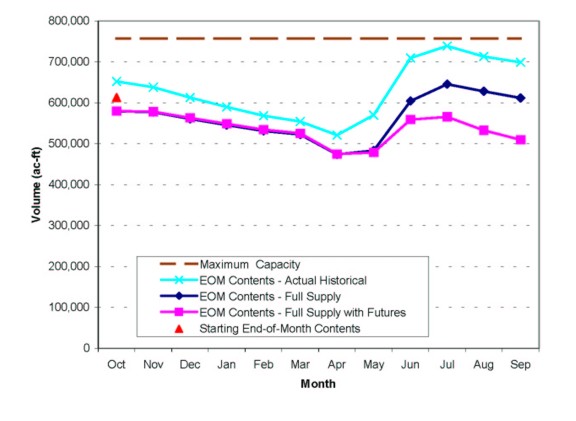
Figure 3.3-1 Simulated End-of-Month Contents for Boysen Reservoir . Average Year
3.3.3 . Streamflow
Streamflow is a fundamental output of any river basin simulation model. The Wind/Bighorn River sub-basin models use streamflow as a calibration measure. This implies that simulated streamflow matches or is very close to measured historical streamflow. Therefore, in Calibration mode, simulated streamflows generally match historical streamflow. As previously discussed, the Wind/Bighorn River sub-basin models are configured to allow the simulation of streamflows given variations in model input parameters, such as diversion requirements. Therefore, for the Full Supply and the Full Supply with Futures Projects scenarios, the impacts to streamflows can be shown. Streamflow impacts at any node within the model can be obtained simply by running the model in the desired modes and comparing the .node inflow. on the reach worksheets at the desired nodes.
3.3.4 . Available Flow
The available surface water for each basin is defined as the amount of water available for water development after meeting downstream demands. These demands include:
Available flows under the Full Supply scenario for the Wind River Basin, Bighorn River Basin and Clarks Fork, Yellowstone and Madison/Gallatin River Basins are shown in Table 3.3-3, Table 3.3-4 and Table 3.3-5. Available flows under the Full Supply with Futures Projects scenario for the Wind River Basin are shown in Table 3.3-6. As previously mentioned, the model does not show any affects on streamflow due to the Futures Projects (see model constraints). The development of available flows is discussed in the following sub-sections.
Table 3.3-3 Wind River Basin Available Flow - Full Supply Scenario
| Basin | Location | Available Flow (ac-ft) | ||
| Dry | Normal | Wet | ||
| Upper Wind | Reach 100: Wind River Headwaters to DuNoir Creek | 0 | 32,973 | 61,735 |
| Reach 200: Wind River from DuNoir Creek to East Fork | 0 | 52,255 | 82,993 | |
| Reach 300: Wind River from East Fork to Bull Lake Creek | 74,745 | 249,772 | 470,811 | |
| Reach 290: East Fork Wind River | 2,586 | 25,922 | 52,810 | |
| Reach 320: Dinwoody Creek | 5,550 | 40,388 | 64,188 | |
| Reach 390: Bull Lake Creek | 14,327 | 107,703 | 161,938 | |
| Little Wind | Reach 400: Wind River from Bull Lake Creek to Little Wind | 98,817 | 312,982 | 528,328 |
| Reach 500: Little Wind River | 26,825 | 88,499 | 137,008 | |
| Reach 510: South Fork Little Wind | 7,454 | 15,620 | 39,709 | |
| Reach 520: North Fork Little Wind | 11,641 | 62,887 | 94,835 | |
| Reach 530: Trout Creek | 2,833 | 5,717 | 8,317 | |
| Reach 580: Popo Agie River | 26,825 | 88,499 | 137,008 | |
| Lower Wind | Reach 600: Wind River from Little Wind Confluence to Boysen Reservoir | 332,085 | 748,665 | 987,068 |
| Reach 700: Muddy Creek | 2,676 | 3,441 | 4,131 | |
| Reach 800: Badwater Creek | 22,101 | 22,007 | 18,305 | |
Notes:
(1)Available Flow in Upper Wind River Basin affected by Instream Flow requirements in Reach 200. The East Fork Wind River is downstream of this Instream Flow segment. However, due to model construction, its impacts are imposed on the East Fork.
Table 3.3-4 Bighorn River Basin Available Flow . Full Supply Scenario
| Basin | Location | Available Flow (ac-ft) | ||
| Dry | Normal | Wet | ||
| Upper Bighorn | Reach 100: Bighorn River to Owl Creek | 758,909 | 1,103,618 | 1,451,214 |
| Reach 400: Bighorn River from Owl Creek to Gooseberry Creek | 775,972 | 1,117,130 | 1,496,273 | |
| Reach 460: Cottonwood Creek | 7,275 | 14,338 | 30,873 | |
| Reach 480: Gooseberry Creek | 7,926 | 14,601 | 22,515 | |
| Reach 500: Bighorn River from Gooseberry Creek to Nowood River | 840,185 | 1,266,937 | 1,659,049 | |
| Reach 900: Bighorn River from Nowood River to USGS Gage | 871,488 | 1,303,478 | 1,694,604 | |
| Owl Creek | Reach 200: Owl Creek from N. & S. Fork Conf. To Mud Creek Conf. | 5,477 | 17,269 | 26,746 |
| Reach 220: South Fork Owl Creek | 1,468 | 9,521 | 16,013 | |
| Reach 250: N. Fork Owl Creek | 1,737 | 6,678 | 11,483 | |
| Reach 300: Owl Creek from Mud Creek Conf. To Bighorn River | 8,907 | 27,540 | 48,091 | |
| Nowood | Reach 600: Nowood River above Ten Sleep Creek | 6,500 | 15,214 | 25,902 |
| Reach 690: Ten Sleep Creek | 3,114 | 12,235 | 24,183 | |
| Reach 700: Nowood River from Ten Sleep Ck. To Paint Rock Ck. | 146,433 | 169,466 | 251,569 | |
| Reach 790: Paint Rock Creek | 82,113 | 91,162 | 112,187 | |
| Reach 800: Nowood River from Paint Rock Ck. To Bighorn Riv. | 248,827 | 295,779 | 424,924 | |
| Lower Bighorn | Reach 1000: Bighorn River at Greybull River | 915,630 | 1,438,245 | 1,797,531 |
| Reach 1500: Bighorn River at Shell Creek | 917,826 | 1,463,859 | 1,829,238 | |
| Reach 1600: Shell Creek | 19,218 | 46,793 | 57,027 | |
| Reach 1700: Bighorn River at Yellowtail | 919,801 | 1,567,955 | 1,911,814 | |
| Reach 1740: Crystal Creek | 1,025 | 2,812 | 6,807 | |
| Greybull | Reach 1100: Greybull River Headwaters | 29,634 | 85,629 | 74,207 |
| Reach 1200: Wood River | 66,134 | 84,738 | 104,651 | |
| Reach 1300: Greybull River below Wood River | 39,696 | 94,879 | 86,534 | |
| Reach 1350: Meeteetse Creek | 1,531 | 3,552 | 5,828 | |
| Reach 1400: Greybull River Below Roach Gulch | 48,053 | 108,263 | 96,906 | |
| Shoshone | Reach 1800: South Fork Shoshone River Headwaters | 6,274 | 11,667 | 18,472 |
| Reach 1900: South Fork Shoshone River below Bob Cat Creek | 97,126 | 260,356 | 425,296 | |
| Reach 2000: North Fork Shoshone River Headwaters | 27,097 | 55,797 | 97,618 | |
| Reach 2100: North Fork Shoshone River below Wapati | 156,891 | 348,970 | 560,480 | |
| Reach 2200: Buffalo Bill Reservoir | 196,528 | 403,274 | 636,417 | |
| Reach 2300: Shoshone River below Buffalo Bill Reservoir | 196,528 | 403,274 | 636,417 | |
| Reach 2390: Sage Creek | 0 | 0 | 103 | |
| Reach 2400: Shoshone River below Sage Creek | 302,875 | 521,599 | 749,870 | |
| Reach 2500: Shoshone River below Bitter Creek | 471,534 | 748,196 | 1,082,116 | |
Table 3.3-5 Clarks Fork, Yellowstone and Madison/Gallatin Basin Available Flow - Full Supply Scenario
| Basin | Location | Available Flow (ac-ft) | ||
| Dry | Normal | Wet | ||
| Clarks Fork | Reach 100: Clarks Fork River above Sunlight Creek Confluence | 240,422 | 370,501 | 528,966 |
| Reach 190: Sunlight Creek | 48,383 | 70,615 | 86,899 | |
| Reach 200: Clarks Fork River from Sunlight Creek to Bennett Creek | 240,422 | 370,501 | 567,608 | |
| Reach 300: Clarks Fork River below Bennett Creek Confluence | 294,923 | 444,004 | 681,550 | |
| Yellowstone | Reach 400: Yellowstone River above Lamar River Confluence | 813,647 | 1,146,594 | 1,328,581 |
| Reach 500: Yellowstone River below Lamar River Confluence | 1,531,126 | 2,140,310 | 2,469,129 | |
| Reach 580: Gardner River | 65,111 | 113,663 | 144,366 | |
| Madison/Gallatin | Reach 600: Madison River | 340,745 | 375,009 | 437,417 |
| Reach 620: Gibbon River | 89,203 | 109,391 | 135,155 | |
| Reach 640: Firehole River | 251,542 | 265,618 | 302,261 | |
| Reach 800: Gallatin River | 501,921 | 634,324 | 716,471 | |
Table 3.3-6 Wind River Basin Available Flow - Full Supply with Futures Projects Scenario
| Basin | Location | Available Flow (ac-ft) | ||
| Dry | Normal | Wet | ||
| Upper Wind | Reach 100: Wind River Headwaters to DuNoir Creek | 0 | 28,187 | 43,626 |
| Reach 200: Wind River from DuNoir Creek to East Fork | 0 | 47,469 | 62,968 | |
| Reach 300: Wind River from East Fork to Bull Lake Creek | 70,387 | 150,190 | 354,645 | |
| Reach 290: East Fork Wind River | 2,586 | 21,858 | 36,403 | |
| Reach 320: Dinwoody Creek | 5,550 | 37,336 | 57,003 | |
| Reach 390: Bull Lake Creek | 14,327 | 70,862 | 111,811 | |
| Little Wind | Reach 400: Wind River from Bull Lake Creek to Little Wind | 91,783 | 214,625 | 406,565 |
| Reach 500: Little Wind River | 26,825 | 88,499 | 137,008 | |
| Reach 510: South Fork Little Wind | 7,454 | 15,620 | 39,709 | |
| Reach 520: North Fork Little Wind | 11,641 | 62,887 | 94,835 | |
| Reach 530: Trout Creek | 2,833 | 5,717 | 8,317 | |
| Reach 580: Popo Agie River | 26,825 | 88,499 | 137,008 | |
| Lower Wind | Reach 600: Wind River from Little Wind Confluence to Boysen Reservoir | 292,772 | 684,113 | 878,067 |
| Reach 700: Muddy Creek | 2,676 | 3,441 | 4,131 | |
| Reach 800: Badwater Creek | 22,101 | 22,007 | 18,305 | |
Notes:
(1)Available Flow in Upper Wind River Basin affected by Instream Flow requirements in Reach 200. The East Fork Wind River is downstream of this Instream Flow segment. However, due to model construction, its impacts are imposed on the East Fork.
Available Flow in Excess of Existing Demands
The Wind/Bighorn sub-basin models are divided into reaches that represent an individual reach of stream. The available flow is calculated as the minimum of the available flow within the individual reach and the available flow of all downstream reaches.
In previous river basin planning models, the available flow within each reach was calculated as the minimum of the outflow from the reach (HKM, 2002). However, it was found that in the Wind/Bighorn sub-basin models, some of the reach outflows were greater than the minimum flow within the reach. Thus, the defining flow availability is the minimum flow within the reach, taking into account compact requirements for the WBHB and instream flow requirements within the reach. Therefore, for the Wind/Bighorn available flows, the available flow within each reach was taken as the minimum flow at all nodes within the reach. The minimum flow for the individual reach was then calculated as the minimum flow within the reach plus the minimum flow of all downstream reaches.
It should be noted that performing these calculations on an annual basis could result in different results than performing the calculations on a monthly basis. The monthly basis is considered more accurate because of the shorter calculation time period. The annual value of available flow is the sum of the 12 months. available flow.
Compact Constraints
The Yellowstone River Compact, which was ratified in 1950 by the states of Wyoming, Montana and North Dakota, governs the allocation of the tributaries to the Yellowstone River between the states. The following is a brief summary of the rules for dividing water according to the Compact (WWDC, 2002):
The information used in this study to determine the volume of availability under the Yellowstone River Compact is based upon conversations and information from the U.S. Geological Survey and with the Wyoming State Engineer.s Office (SEO) (YRCC, 2002). For the Clarks Fork of the Yellowstone River, the Compact allocates 60 percent of the unallocated flows to Wyoming and 40 percent to Montana. For the Bighorn River, the Compact allocates 80 percent of the unallocated flow to Wyoming and 20 percent to Montana. A summary of the annual unallocated flow calculations using the methodologies prescribed by the Compact Commission are shown in Table 3.3-7.
Table 3.3-7 Calculation of Wyoming Portion of Unallocated Flow
| Clarks Fork | Bighorn River | |||||
| Dry Year | Normal Year | Wet Year | Dry Year | Normal Year | Wet Year | |
| Gaged Flow (ac-ft) | 491,713 | 733,406 | 1,137,418 | 1,911,049 | 2,778,269 | 3,591,471 |
| Adjusted Flow (ac-ft) | 498,664 | 740,007 | 1,144,083 | 1,686,523 | 2,559,384 | 3,382,968 |
| Wyoming Portion of Unallocated Flow (ac-ft) | 299,199 | 444,004 | 686,450 | 1,349,218 | 2,047,507 | 2,706,375 |
| Wyoming Portion of Unallocated Flow (ac-ft) minus Futures Projects | N/A | N/A | N/A | 1,099,218 | 1,797,507 | 2,456,375 |
Notes:
(1)Based on 1973 . 2001 data.
Instream Flow Conditions
The Wyoming Water Development Commission (WWDC) applies for instream flow permits for fishery uses within the stream reach. Within the Wind/Bighorn Basin Plan study area, there are three streams with permitted instream flows, one stream with two separate reaches, and two streams with pending instream flow applications. The permitted and pending instream flow reaches and flow rates are shown in Table 3.3-8 (Brinkman, 2002). The instream flows are more fully discussed in the Technical Memorandum Recreational and Environmental Uses and Demand (BRS, 2002).
Table 3.3-8 Permitted and Pending Instream Flow Rates
| Instream Flow Segment | Model Reach | Permitted/Pending Instream Flow (cfs) | |||||||||||
| Jan | Feb | Mar | Apr | May | Jun | Jul | Aug | Sep | Oct | Nov | Dec | ||
| Clarks Fork | 200 | 200 | 200 | 200 | 200 | 200 | 200 | 200 | 200 | 200 | 200 | 200 | 200 |
| Tensleep | 690 | 22 | 22 | 22 | 22 | 22 | 22 | 22 | 22 | 22 | 22 | 22 | 22 |
| Big Wind | 200 | 102 | 102 | 102 | 110 | 110 | 102 | 102 | 102 | 102 | 102 | 102 | 102 |
| Shell 1(1) | 1600 | 19 | 19 | 19 | 45 (1) | 70 | 70 | 40 | 40 | 40 | 19 | 19 | 19 |
| Shell 2 | 1600 | 23 | 23 | 23 | 23 | 23 | 23 | 40 | 40 | 40 | 23 | 23 | 23 |
| Medicine Lodge Creek (2) | 794 | 8.9 | 8.9 | 8.9 | 8.9 | 8.9 | 8.9 | 8.9 | 8.9 | 8.9 | 15 | 15 | 8.9 |
| Shoshone River (2) | 2300 | 350 | 350 | 350 | 350 | 350 | 350 | 350 | 350 | 350 | 350 | 350 | 350 |
Notes:
(1)The flow requirement in April for Shell No. 1 is 19 cfs April 1-15 and 70 cfs April 16-30. The calculations assume the average of these two values for the April value.
(2)The Medicine Lodge Creek and Shoshone River instream flow applications are pending.
Instream flows exert a demand on the river the same as any other consumptive use water right. Flow must be passed through the instream flow segment according to the water right priority date. Once that flow is through the segment, the water can be diverted for consumptive use. Therefore, available flows for reaches upstream of the permitted instream flow rights are affected assuming that water rights for use of the available flows would be junior to the instream flow rights.
All available flow calculations assume that both the permitted and pending instream flow water rights are in place. Therefore, any upstream flows that are not in excess of the instream flow right are shown to be unavailable for future uses. Each of the instream flow segments is within a modeled reach as shown in the table. For purposes of the calculations, it was assumed that the entire reach is subject to the instream flow requirement even if the instream flow segment occupies only a small portion of the reach. The reaches most affected by the instream flow water rights are the Upper Wind River, Shell Creek, Medicine Lodge and Tensleep Creek, especially in the winter months. Flows in Medicine Lodge Creek are a concern primarily during the summer when flows in the instream flow reach typically drop very low.
3.4 . Available Ground Water Determination
3.4.1 . Introduction
This section provides a qualitative summary of the ground water resources of the Wind, Bighorn, Yellowstone, Clarks Fork, Gallatin, and Madison River Basins of north-central Wyoming. Additional information is provided in the Technical Memorandum, Available Ground Water Determination, Chapter 3, Tab 17, for the Wind/Bighorn River Basin Plan. In completion of this study, no original investigations were performed. The study represents an inventory, compilation, and review of published literature on the geology and ground water resources of the planning area.
Study Objectives
The first objective was to inventory and document existing published data on ground water studies and ground water planning documents for the planning area. A listing of related ground water studies is provided in Appendix A, of the technical memorandum, Chapter 3, Tab 17. Most of the existing ground water studies and ground water planning documents have considered the planning area with respect to either individual counties or as separate geographic areas such as the Wind River Basin, the Bighorn Basin, and the Yellowstone Plateau. Additional information on specific geographic areas within the planning area is available through the U.S. Geological Survey (USGS), the U.S. Bureau of Land Management (BLM), and other federal agencies.
A second objective was to inventory and catalog the SEO ground water permit database for various categories of ground water uses in the planning area, and incorporate the extracted information into four GIS data layers. This was accomplished through a cooperative effort of personnel of the SEO and WWDC. GIS data layers prepared from information on file with the SEO as of December 31, 2001, are presented in Appendix B, of the technical memorandum, Chapter 3, Tab 17, and include:
A third objective of this investigation was to semi-quantitatively assess the impacts of well interference in more intensively developed ground water production areas near Hyattville and Riverton. The Wind River Aquifer near Riverton has been extensively developed primarily for municipal and domestic use. In the vicinity of Ten Sleep and Hyattville, the Tensleep, Madison, and Flathead Aquifers have been developed principally for agricultural use, but are also used for municipal and industrial purposes. These particular areas were investigated at the request of WWDC personnel to assess whether or not a control area designation may be warranted at this time.
Other objectives include:
3.4.2 . Geological Setting
Encompassing approximately one quarter of the state, the planning area contains a wide variety of geologic formations and structural elements within the Wind River Basin, the Bighorn Basin, and the Yellowstone Plateau. Geologic formations vary in thickness and in age from Precambrian crystalline rocks to recent alluvial and terrace deposits of silts, clays, sands, and gravels. The Wind River Basin contains roughly 18,000 feet of Cenozoic through Paleozoic sedimentary strata (Richter, 1981). Similarly, the Bighorn Basin contains approximately 33,000 feet of Cenozoic through Paleozoic sediments (Libra and others, 1981). In contrast, the Yellowstone Plateau and mountain ranges to the east contain at least 15,000 feet of Cenozoic volcanics and volcanic sediments that overlie Mesozoic and Paleozoic sedimentary rocks (Cox, 1976). General surficial and bedrock geology of the planning area is shown on Figures 3.4-1 and 3.4-2.
The Wind River and Bighorn Basins are both large asymmetrical structural depressions that contain up to 18,000 and 33,000 feet, respectively, of Cenozoic, Mesozoic, and Paleozoic sediments that rest unconformable on Precambrian crystalline basement rocks (Libra and others, 1981; Richter, 1981). With the exception of the western Bighorn Basin that is covered with Absaroka Volcanics, these structural Basins are bordered by compressional uplifts of Precambrian granite cores mantled by moderately to steeply dipping sedimentary formations (Libra and others, 1981). While it has been speculated that these or similar structures extend far into Yellowstone National Park, the Yellowstone Plateau coincides with a large volcanic caldera (Cox, 1976; Libra and others, 1981). The configuration of these geologic formations and structural elements greatly influence the occurrence and availability of ground water in the planning area.
Within the Bighorn and Wind River Basins, significant quantities of oil, gas, and uranium have been commercially developed from sedimentary rocks. Coal and bentonite have both been commercially developed within the Bighorn Basin. Most oil and gas in the region has been developed from Mesozoic and Paleozoic rocks in structurally sympathetic anticlines (Richter, 1981; Libra and others, 1981). The Wyoming Oil and Gas Conservation Commission (2000) reported approximately 20 million barrels of oil and 156 million cubic feet of natural gas were produced from 4,937 wells in Big Horn, Fremont, Hot Springs, Park, and Washakie Counties in 2000. Uranium has been produced from the Wind River Formation in the Wind River Basin.
3.4.3 . Hydrostratigraphy
An aquifer is generally defined as a geologic formation or group of formations that are sufficiently saturated and permeable enough to yield a significant quantity of water to wells or springs. Of the more than 40 geologic formations that are present in the planning area, at least 12 aquifers and two aquifer systems have been recognized (Richter, 1981; Libra and others, 1981). The two aquifers primarily developed for high capacity municipal supply are the Wind River and Madison Aquifers.
For this report, the formations have been grouped into 13 principal aquifers that have historically been the major ground water sources for development. The grouping was based on that presented in the 1981 reports on the "Occurrence And Characteristics of Ground Water in the Wind River Basin, Wyoming," and on the .Occurrence And Characteristics of Ground Water in the Bighorn Basin, Wyoming,. by the Wyoming Water Resources Research Institute (WWRI) (Richter, 1981; Libra and others, 1981). Figure 3.4-3 graphically summarizes the hydrogeologic role of the geologic formations in the area.
The WWRI aquifer division used herein was based on the hydrogeologic character of the geologic formations of Richter (1981). While more detailed than the description of Libra and others (1981), the division allows for a more accurate, regional presentation of the principal sources of ground water in the planning area. The 13 major aquifers are (youngest to oldest):
As previously mentioned, the two aquifers primarily developed for high capacity municipal supply are the Wind River and Madison Aquifers. The Wind River Aquifer is composed of sufficiently saturated and permeable sandstone and conglomerate of the Wind River Formation, and it is the major source of drinking water for domestic and water supply purposes in the vicinity of Riverton and Shoshoni in the Wind River Basin. Although these lenticular sandstone and conglomerate beds are difficult to correlate, aquifer tests of the Riverton Municipal Well Field and the Fremont Minerals deep well in Riverton have revealed the entire sandstone, siltstone, and shale sequence of the Wind River Formation is sufficiently hydraulically connected (Gores and Associates, 1998). Nevertheless, the presence of these shales and siltstones has resulted in a series of semi-confined and confined sandstone subaquifers. Approximately 1,700 wells had been drilled into the Wind River Aquifer as of 1981. These wells reportedly yield water from both unconfined and confined sandstone beds (Richter, 1981).
The Madison Aquifer is composed of sufficiently saturated and permeable portions of the Madison Limestone, Darby Formation, and Bighorn Dolomite, and it is a primary source of drinking water for several municipalities in the Bighorn Basin. The Madison Limestone and Bighorn Dolomite are thick-bedded carbonate rocks that include considerable chert. Cooley (1986) noted that in most outcrops Madison and Bighorn strata are transected by many large vertical fractures, which can make drilling difficult and cause the loss of drilling fluid circulation. Along the crests of anticlinal folds in which through-going vertical joints provide conduits for vertical flow, the Madison Aquifer is locally hydraulically connected to the overlying Tensleep Aquifer (Cooley, 1986). Yield from the Madison Aquifer is contingent upon the number of permeable interconnected fractures or solution tubes encountered in individual wells.
3.4.4 . Ground Water Quality
Water quality conditions in the aquifers of the planning area were extensively reviewed by the USGS during the preparation of county water resources reports during the 1990s, and by the Wyoming Water Resources Research Institute in the early 1980s. This research indicated the best quality ground water is usually derived from areas closest to the geologic outcrop areas of each aquifer. Generally, the water quality of ground water derived from each aquifer is variable and dependent upon a variety of factors including, but not necessarily limited to the following: distance from the recharge area, aquifer transmissivity and storage, ground water flow rates, aquifer rock type, dissolution of soluble salts within the aquifer matrix, and leakage of poor quality water from adjacent units (Richter, 1981).
Water Quality Standards and Suitability for Use
The State of Wyoming has identified the following standards for different classes of ground water (WDEQ, 1993):
While used for municipal and domestic supply in the Basin, ground water has historically been used primarily for agricultural and industrial purposes (Richter, 1981; Libra and others, 1981). Ground water used for agricultural purposes has principally been used for cropland irrigation, but stock watering has also been a major component. While the production of uranium and iron ore has beneficially used ground water resources, the most significant industrial production of ground water has been for petroleum recovery. With the adoption of the Surface Water Treatment Rule, ground water not directly affected by surface water has become an attractive target for primary or supplementary supply sources in the planning area, particularly for Greybull, Manderson, Basin, Worland, and Riverton. Other municipalities, including Lander and Thermopolis, are currently exploring this option as well. A relatively small percentage of ground water is also used for environmental and recreational purposes. Ground water used for these purposes is used to supply water to fish hatcheries, campgrounds, a golf course, state and national parks, and private hot springs resorts. Although its quality can vary widely over the planning area, ground water remains a very valuable source of water for many people, livestock, and industries. The key to its satisfactory development is directly related to the primary purpose for which the ground water will be used in accordance with the above list of bulleted ground water classes.
Aquifer Sensitivity/Vulnerability
The University of Wyoming's Spatial Data and Visualization Center (SDVC) developed a system to assess the sensitivity and vulnerability of ground water to surface water contamination in Wyoming (Hamerlinck and Arneson, 1998a). Potential sources of contamination in the planning area include railroad and highway transportation routes, oil and gas pipelines that traverse the Basin, oil and gas wells and well fields, hazardous waste spills, agricultural chemicals applied to farmlands, mining related chemicals and wastes, and underground injection wells. Development of the system was made possible through EPA Section 319 Program funding. Additional financial support was provided by the Wyoming Non-Point Source Task Force, USEPA Region VIII, and the Wyoming Department of Environmental Quality, Water Quality Division. The Wyoming Department of Agriculture also provided support and guidance in the initial planning phase to develop the assessment system (Hamerlinck and Arneson, 1998a).
With the exception of the Yellowstone National Park area, the SDVC developed aquifer sensitivity maps to define the potential for surface contamination to impact ground water in the uppermost aquifer throughout Wyoming. Plate D.1, Appendix D, technical memorandum, Chapter 3, Tab 17 is a map of aquifer sensitivity to contamination within the planning area. Lands rated as being most sensitive to contamination generally are located on alluvial deposits adjacent to rivers, streams, and lakes; on slope wash, colluvium, residium, and eolian deposits; and on fractured bedrock areas.
Plate D.2, Appendix D, technical memorandum, Chapter 3, Tab 17, is a map of aquifer vulnerability to pesticide contamination for the uppermost or shallowest aquifers in the area. Ground water is vulnerable in areas with high water tables, sandy soils, and areas of presumed pesticide application. Areas with the highest vulnerability are also generally located in the floodplains of major streams or are associated with slope wash, colluvium, residium, and eolian deposits.
3.4.5 . Ground Water Development
Within the limits of the planning area, ground water is the primary source of water for many uses. While the Madison and Wind River Aquifers represent the most utilized sources of municipal supply, all 13 aquifers are important water sources for different reasons throughout the planning area.
Existing Development
The 12,381 active ground water permits inventoried by the SEO as of December 31, 2001, demonstrate the overall significance of ground water resources in the planning area. From these wells, two GIS database layers were prepared to show the locations of non-domestic wells that have water rights of greater than 50 gpm. Two maps showing the locations of all permitted domestic wells were also prepared. The following bulleted list summarizes the number of wells for each usage category that were used in the preparation of the GIS data layers:
The locations of these wells are presented with respect to surficial and bedrock geology, and usage type in Plates B.1 through B.4, Appendix B, Technical Memorandum, Chapter 3, Tab 17. Review of the plates provides a general understanding of the overall significance of individual aquifers based on the type of use, well depth, geologic formation outcrop areas, and geographic location.
Within the planning area, the SEO has permitted approximately 222.6 million gallons per day (MGD) of ground water for various uses. While this amount does not indicate average daily usage, it does reveal the magnitude of existing ground water development in the area. The following paragraphs further discuss existing ground water development according to the type of use.
Agricultural wells in the Basin are used to deliver approximately 88.5 MGD or 39.7% of the total. Most of these wells are used to irrigate croplands or hayfields along either the margins of the Basin or along alluvial channels.
The second largest use of ground water in the Basin, industry uses approximately 63.3 MGD or 28.4% of the total. Petroleum and mineral development companies are the major developers of ground water in this area. In fact, the Wyoming Oil and Gas Conservation Commission (2000) reported approximately 108 MGD of ground water were produced from 4,937 wells in Big Horn, Fremont, Hot Springs, Park, and Washakie Counties in 2000. It is uncertain how much of this quantity was actually consumed, however, and it is presumed that most of this water was used to enhance oil or gas recovery.
Based on information provided to the WWDC, municipalities in the Basin use 3.9 MGD of ground water on average and a maximum of 8.8 MGD. This ground water is consumed by 36 municipal and non-municipal community public water systems that are located in the Basin. By contrast, the SEO has already issued permits for 54.2 MGD of ground water development, which suggests either that the SEO believes there are sufficient quantities of ground water still available for development, or that more water is being used than is being reported.
Domestic ground water use in the Basin was estimated on the basis of the rural population, which predominately uses ground water for domestic supply. While the total population of the planning area as of 2000 has been estimated to be 85,222 people, the population of municipalities and those served by public water systems has been estimated to be approximately 59,000. To quantify the amount of ground water used for domestic purposes, the population served by municipal systems was subtracted from the total population for the area, or 26,222 people. An estimated per capita usage rate of 75 gallons per day was used to estimate daily usage. Based on this method, approximately 1.96 MGD of ground water are used to supply the rural population of the planning area.
Ground water is also used for recreational and environmental purposes in the Basin. This ground water is used to supply fish hatcheries, campgrounds, and private recreational facilities. Approximately 4.78 MGD of the total are used for recreational purposes, while 4.15 MGD are used for environmental purposes. Actual consumptive use is likely much less than these figures.
Impacts of Existing Development
The Wind River Aquifer near Riverton has been extensively developed primarily for municipal and domestic use. In the vicinity of Ten Sleep and Hyattville, the Tensleep Aquifer, Madison Aquifer, and the Flathead Sandstone have been developed not only for agricultural use, but are also used for municipal and industrial purposes. These particular areas were investigated to assess whether or not a control area designation may be warranted at this time.
According to Wyoming Water Statute § 41-3-912, a control area can be designated by the Board of Control upon the initiative of the State Engineer for the following reasons:
Based on SEO records, approximately 48 wells with water rights in excess of 50 gpm have been drilled within the area around Ten Sleep and Hyattville since 1945, as shown on Plate E.1 found in appendix B of chapter 3 of the Technical Memorandum. Most of these wells were completed in either the Madison Aquifer or the Flathead Sandstone and are flowing artesian. Used for municipal purposes, the City of Worland wells, Husky No. 1 and Worland No. 3, have the largest water rights of any wells in the area at 5,000 and 6,660 gpm respectively. In combination with the other seven municipal and quasi-municipal wells in the area, approximately 13,800 gpm of water rights have been allocated for municipal use in the area. The second largest use of ground water in the area is irrigation. This area contains eleven wells that are each permitted to produce more than 400 gpm, and are yield a combined total of approximately 13,300 gpm.
The overall impact of existing ground water development from the Paleozoic Aquifers in the vicinity of Ten Sleep and Hyattville appears to vary with time and by geographic location. In arriving at this conclusion, wellhead pressures and water level data were obtained through a June 18, 2002, meeting with local agricultural users, and by contacting Worland, Hyattville, Ten Sleep, the South Bighorn Regional Joint Powers Board, and the SEO. Cooley (1986) and Susong and others (1993) reported that periodic data from various wells in the area were collected by the USGS in 1953, 1962, 1970, 1975-1978, and 1989. While Cooley (1986) reported a decrease in the wellhead pressure of Ten Sleep No. 1 in Section 16 of T47N, R88W, between 1972 and 1977 corresponded to decreased combined flow from a well and spring at the Wigwam Fish Rearing Station east of Ten Sleep, recent data from this well and Ten Sleep No. 2 in Section 17 of T47N, R88W, suggest the static artesian pressure of the Madison Aquifer at this location has not declined. In contrast, Madison Aquifer artesian pressures appear to be declining in the vicinity of Worland.s wells in T49N, R91W near Hyattville, as shown on Plate E.1, Technical Memorandum, Chapter 3, Tab 17. Wellhead pressures for wells completed in the Flathead Sandstone also continue to decline due to continuous production via irrigation or interaquifer leakage (Susong and others, 1993).
In contrast to the Ten Sleep and Hyattville vicinity, ground water from the Wind River Aquifer in the vicinity of Riverton is almost exclusively used for municipal or quasi-municipal purposes. Of the roughly 1,010 ground water permits issued by the SEO near Riverton, approximately 98% are used for municipal or domestic use (Gores and Associates, 1998). Only 44 of these permits are for ground water production of 50 gpm or more, and 23 of the 25 wells that are permitted for 100 gpm or more are completed at depths of 300 feet or greater. According to the SEO, all 13 of Riverton.s municipal supply wells are completed at depths of 300 feet or greater. Gores and Associates (1998) reported these wells are permitted to yield a total of 4,015 gpm. The average production of these wells between 1987 and 1996 was 710 gpm.
Water level records maintained by the City of Riverton and the USGS indicate ground water levels in the Wind River Aquifer have been lowered as a result of municipal ground water production since 1924, as shown on Plate E.2, Technical Memorandum, Chapter 3, Tab 17. While monthly production records for Riverton.s well field are only available since July 1957, these records reveal that ground water production steadily increased from 632 to 1,357 gpm per year between 1958 and 1980. Annual well production dropped to approximately 696 gpm following the City.s installation of a surface water treatment plant in June 1981 (Gores and Associates, 1998). Although demands on the Wind River Aquifer between May and September have been reduced through the treatment and use of surface water from the Wind River, water levels in the Riverton area remain well below those of the 1940s. In the vicinity of the inactive municipal wells in southwestern Riverton, water levels are approximately 60 feet below 1940s levels based on static water levels reported on well completion reports, and water levels in the vicinity of Riverton.s current production wells are well over 90 feet lower (Gores and Associates, 1998). Furthermore, Riverton.s long reliance upon the storage capabilities of the aquifer has resulted in an area-wide lowering of the water level by approximately 30 feet.
Based on recorded declines in water levels and wellhead pressures in these areas near Hyattville and Riverton, the SEO may want to further investigate these areas and talk with local residents regarding the necessity of establishing control areas at these locations.
Future Development
Geologic conditions, drilling depths, hydrogeologic characteristics, and the ground water quality of the numerous aquifers vary throughout the planning area. Depending upon the proposed type of use and required water quantities, virtually all of the aquifers probably have some potential for development. Site specific investigations and experience will be required to assess specific possibilities to develop ground water from wells with sufficient capacity for a specific use.
While numerous hydrogeological investigations have been conducted in the planning area, there have been few, if any, regional assessments of the annual recharge, storage, and sustained yield capability of the major aquifers. General conclusions regarding the ground water development potential of several of the major aquifers are summarized below:
Table 2 in the Wind/Bighorn Technical Memorandum Available Ground Water Determination, Technical Memorandum, Chapter 3, Tab 17, summarizes the development potential of each aquifer within the planning area, along with its general lithologic and hydrologic character, and its general ground water quality.
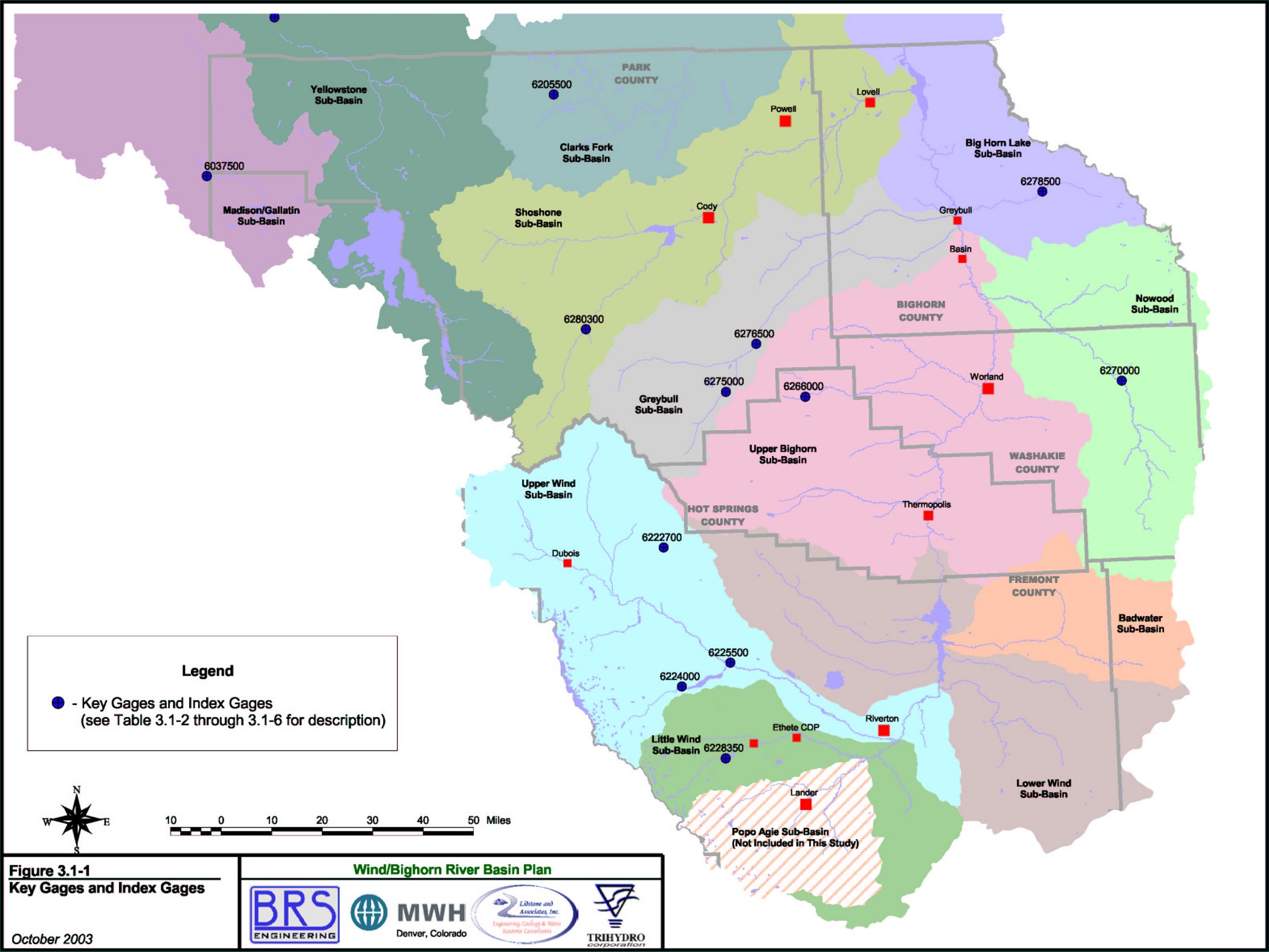
(Click on image to enlarge)
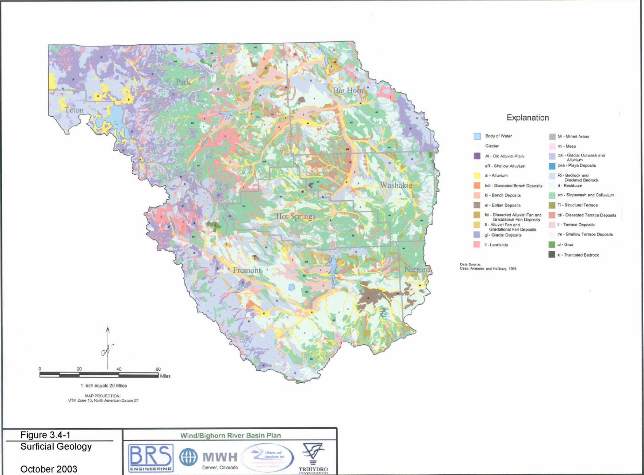
(Click on image to enlarge)
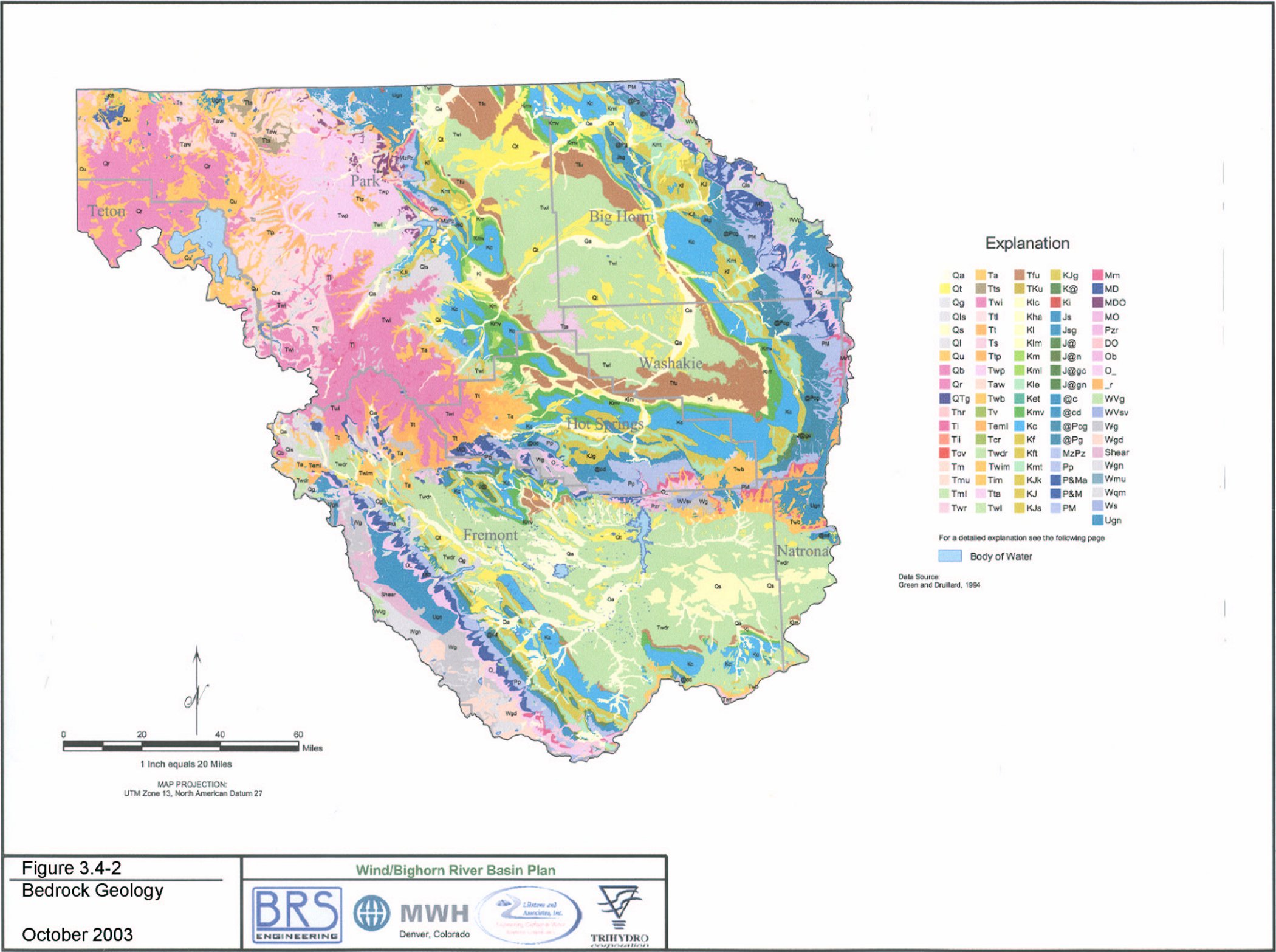
(Click on image to enlarge)
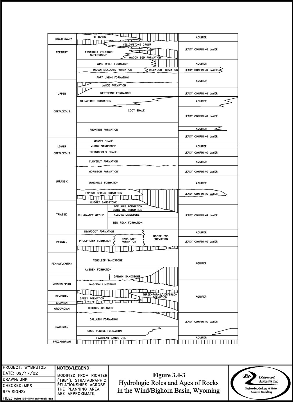
(Click on image to enlarge)