Wyoming State Water Plan
Wyoming State Water Plan
Wyoming Water Development Office
6920 Yellowtail Rd
Cheyenne, WY 82002
Phone: 307-777-7626

Wyoming Water Development Office
6920 Yellowtail Rd
Cheyenne, WY 82002
Phone: 307-777-7626
| SUBJECT: |
Appendix P Surface Water Spreadsheet Model Development |
| PREPARED BY: | Bear River Basin Planning Team |
| DATE: | September 18, 2000 |
1.0 Introduction
The Wyoming Water Development Commission has undertaken statewide water basin planning efforts in selected river basins. The purpose of the statewide planning process is to provide decision makers with current, defensible data to allow them to manage water resources for the benefit of all the state's citizens. The Bear River, because of its interstate nature, has been selected as an initial basin to catalogue its water resources.
The Bear River Spreadsheet Model is a complex spreadsheet which incorporates multiple diversions, reservoirs, gaging stations, and other water resources within the Bear River located in the extreme southwest corner of Wyoming. The model was developed following several months of effort and coordination with various state and local agencies and water officials. The purpose of the model is to provide a planning tool to the State of Wyoming for use in determining those river reaches in which flows may be available to Wyoming water users for future development.
1.1 Model Overview
Individual spreadsheet models were developed which reflect each of three hydrologic conditions: dry, normal, and wet year water supply. Each model relies on historical data from the 1971 to 1998 study period to estimate the hydrologic conditions, as discussed in the Task "A Memorandum, ASurface Water Data Collection and Study Period Selection." Such factors as streamflow, diversions, and irrigation returns were analyzed to determine the type of hydrologic condition and are the basic input data to the model. The model does not explicitly account for water rights, appropriations, or compact allocations nor operate the river basin based on these legal constraints. It is assumed that the historic data reflect effects of any limitations which may have been placed upon water users by water rights restrictions.
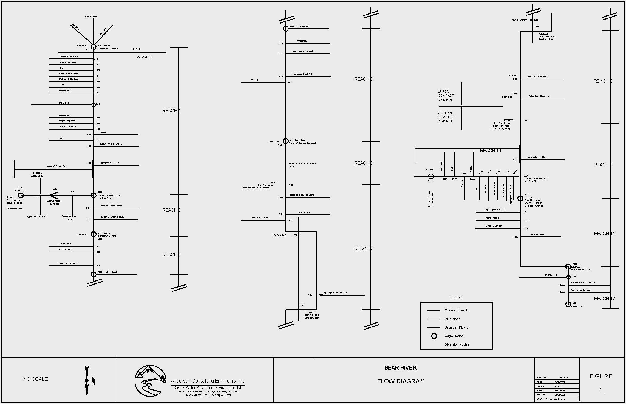
To mathematically represent the Bear River system, the river system was divided into twelve reaches based primarily upon the location of USGS gaging stations. Other key locations, such as reservoirs or confluences with major tributaries, were also used to determine the extent of reaches. Each reach was then sub-divided by identifying a series of individual nodes representing locations where diversions occur, basin imports are added, tributaries converge, or other significant water resources features are located. Figure 1 presents a node diagram of the model developed for the Bear River.
At each node, a water budget computation is completed to determine the amount of water that flows downstream out of the node. Total flow into the node and diversions or other losses from the node are calculated. At non-storage nodes, the difference between inflow, including return flows, and diversions is the amount of flow available to the next node downstream. For storage nodes, an additional loss calculation for evaporation and the change in storage are evaluated. Also at storage nodes, any uncontrolled spill which occurs is added to the scheduled release to get total outflow. Mass balance, or water budget calculations, are repeated for all nodes in a reach, with the outflow of the last node being the inflow to the top node in the next reach.
For each reach, ungaged stream gains (e.g., ungaged tributaries, groundwater inflow, and return flows from unspecified diversions) and losses (e.g. seepage, evaporation, and unspecified diversions) are computed as the difference between average historical gage flows. Stream gains are input at the top of a reach to be available for diversion throughout the reach and losses are subtracted at the bottom of each reach.
Model output includes the target and actual diversions at each of the diversion points, streamflow at each of the Bear River Basin nodes, and evaluation of water emergency conditions as defined by the Bear River Compact. Estimates of impacts associated with various water projects can be analyzed by changing input data, as decreases in available streamflow or as changes to diversions occur. New storage projects that alter the timing of streamflows or shortages may also be evaluated. Complete model input and output for each of the dry, normal, and wet year conditions are included in Appendices A, B, and C, respectively.
1.2 Model Development
The model was developed using Microsoft® Excel 2000. It consists of a series of three-dimensional spreadsheets (i.e., workbooks) which can be thought of as a series of water commissioner's worksheets; each page or worksheet contains the data or logic necessary to compute a separate task. Each entry (i.e., cell) in a workbook contains data or formulas which reference other cells on the same page or anywhere within the workbook. The function of each page (i.e., worksheet) is discussed in detail in subsequent sections of this memorandum.
Within the workbooks are macros written in Microsoft® Excel Visual Basic programming language. The primary function of the macros is to facilitate navigation within the workbook. There are no macros which complete computation of any formulas or results. In other words, whenever a number is input into any cell anywhere in the workbook, the entire workbook is recalculated and updated automatically.
The model was developed with the novice Excel user in mind. Every effort has been taken to lead the User through the model with interactive buttons and mouse-driven options. However, an elementary level of expertise in spreadsheet usage and programming is assumed. This document will not provide instructions in the use of Excel for this spreadsheet. Appendix G is provided as a guide to installing the model. Appendix H is provided as a programmer=s guide to assist in editing the Excel code and for future modifications to the model. In the next chapter, information and instructions on the use of the model are detailed.
2.0 Model Structure and Components
Each of the three hydrologically-conditioned Bear River Models is a three-dimensional spreadsheet (workbook) consisting of numerous individual pages (worksheets). Each worksheet is a component of the model and completes a specific task required for execution of the model. There are five basic types of worksheets:
In this chapter, each component of the Bear River Model is discussed in greater detail. A general discussion of each component includes a brief overview of the function. The discussion of each component also generally includes two sections:
Programmer Notes, which are instructions and suggestions for programmers modifying the model, are included in Appendix H. These will assist state and local officials with any modifications of this model to analyze changed conditions or other applications in the Bear River Basin. Additionally, since this model may be a basis for developing spreadsheet models for other basins, this will serve as a guide for other consulting groups.
2.1 The Navigation Worksheets
A Graphical User Interface (GUI) was developed to assist the User in navigating around the spreadsheets. The initial navigation worksheet or GUI provides the User with an interactive interface to the Bear River Model. The GUI provides a brief tutorial, help screens, and information regarding the current model version (Figure 2). It is initialized by opening the Bear River Model file from within Excel. From the GUI, the User may select the appropriate model to evaluate the desired hydrologic condition (i.e., average dry, normal, or wet year).
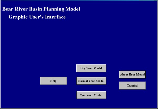
Figure 2. Graphical User's Interface (GUI) Main Page
Each hydrologically-conditioned model, after the GUI interface, has three main navigation worksheets. The Navigation Worksheets assist the User in moving around within the workbook. Each Navigation Worksheet contains buttons which enable the User to view any portion of the workbook. For Users experienced with Excel spreadsheets, all conventional spreadsheet navigation commands are still operative (e.g., page down, GOTO, etc.).User Notes:
Upon opening the Bear River Model file, the User is presented with several options:
1. HELP Provides a text file containing instructions and background information, 2. Dry Year Model: Open the Dry Year Model workbook, 3. Normal Year Model: Open the Normal Year Model workbook, 4. Wet Year Model: Open the Wet Year Model workbook, 5. About Bear River Model: Obtain information pertaining to the current version of the model, 6. Tutorial Open a brief tutorial of the Bear River Model, 7. Close the Bear River Model Close any open workbooks.
2.1.1 The Central Navigation Worksheet
The Central Navigation Worksheet is the "heart" of the model. From here, the User can "jump" to and from any worksheet in the model (Figure 3).
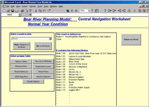
Figure 3. Central Navigation Worksheet
User Notes:2.1.2 The Basin MapThis is the first worksheet the User will see upon selection of a hydrologic condition from the GUI. From this worksheet, the User can access any other worksheet in the model. A series of buttons can be used to "jump" directly to any other location in the workbook. Figure 3 displays the Central Navigation Worksheet from the Normal Year Model.
The User can go to specific reaches by selecting the desired reach from the pull-down menu. When a reach is selected, a table is presented which tabulates all of the nodes in that reach and a brief description of it.
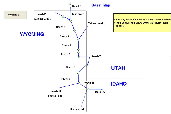
User Notes:2.1.3 The Results NavigatorThe Basin Map Worksheet (Figure 4) provides a simple "stick diagram" of the basin, which is a simplified version of Figure 1. This interactive screen allows the User to visually select a reach to which to "jump". To select a reach, simply click on any reach arrow or its name.
Figure 4. Bear River Basin Diagram (GUI)
User Notes:The Results Navigator (Figure 5) facilitates the selection of any of the following output tabulations:
- Estimated Outflow from each Node
- Estimated Outflow from each Reach
- Estimated Diversions at each Diversion Node
- Estimated Total Diversions from each Reach
- Compact Allocations: Upper Division
- Compact Allocations: Central Division
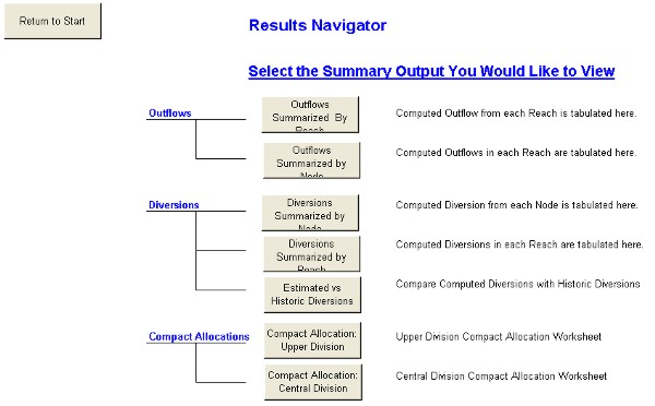
Figure 5. Bear River Basin Results Navigator Worksheet (GUI)
2.2 The Input Worksheets
2.2.1 Master List of Nodes: Matching Number and Name
The model is structured around nodes at which mass balance calculations are made and reaches that connect the nodes. Nodes are points on the river that represent such water resources features as USGS Gage locations, diversion headgates, confluences of the Bear River and its tributaries, or reservoirs. There are a total of 64 nodes in the model; 10 USGS gages, 36 named or key diversion points, 10 aggregated diversion points, and two fully modeled reservoirs (i.e., storage modeled and evaporation included). Also included are five node points, which are confluences of tributaries with the mainstem and Stewart Dam, which was modeled as a river node point but not as a reservoir.
Engineering Notes:2.2.2 Gage DataThe delineation of a river basin by reaches and nodes is more an art than a science. The choice of nodes must consider the objectives of the study and the available data. It also must contain all the water resources feature that govern the operation of the basin. The analysis of results and their adequacy in addressing the objectives of the study are based on the input data and the configuration of the river basin by the computer model.
User Notes:
This worksheet presents a master list of all nodes included in the Bear River Model (Table 1). The list allows the User to view a simple, comprehensive listing of all nodes within the model, organized by reach and node number. This master list governs naming and numbering conventions on many worksheets, so changing the list must be carefully done and checked. Many of the calculations within the spreadsheet are dependent on the proper correlation of node names and numbers.
Note that the numbering convention used for node identification includes the reach number and the location of the node within it. For example, Node 10.05 is the fifth node in Reach 10. There are exceptions to this rule where a node has been added between existing nodes. In these cases, the numbering is not sequential, but the numbering system does not govern the flow connections in the system.
Table 1. Master List of Node Numbers and their Names
Node 1.00 USGS 10011500: Bear River near UT-WY State Line Node 1.01 Lannon & Lone Mountain Node 1.02 Hilliard West Side Node 1.03 Bear Canal Node 1.04 Crown & Pine Grove Node 1.05 McGraw & Big Bend Node 1.06 Lewis Node 1.07 Meyers No. 2 Node 1.08 Meyers No. 1 Node 1.09 Meyers Irrigation Node 1.10 Evanston Pipeline Node 1.11 Booth Node 1.12 Anel Node 1.13 Evanston Water Supply Node 1.15 AggDiv BR-1 Node 2.00 USGS 10015700: Sulphur Cr. ab Res.BL.La Chapelle Cr.Nr. Evanston,WY Node 2.01 AggDiv SC-1/Broadbent Node 2.02 Sulphur Creek Reservoir Node 2.03 AggDiv SC-2 Node 3.00 Confluence Sulphur Creek / Bear River Node 3.01 Evanston Water Ditch Node 3.02 Rocky Mtn & Blyth Node 4.00 USGS 10016900: Bear R. at Evanston, WY Node 4.01 John Simms Node 4.02 S P Ramsey Node 4.03 AggDiv Br-2 Node 5.00 Confluence Yellow Creek / Bear River Node 5.01 Chapman Canal Node 5.02 Morris Bros (Lower) Node 5.03 AggDiv BR-3 Node 5.04 Tunnel Node 6.00 USGS 10020100: Bear R. ab Res. near Woodruff, UT Node 6.01 Woodruff Narrows Reservoir Node 7.00 USGS 10020300: Bear R. bel Res. near Woodruff, UT Node 7.01 Francis Lee Node 7.02 Bear River Canal Node 7.03 Aggregate Utah Diversions Node 8.00 USGS 10026500: Bear R. near Randolph, UT Node 8.01 Pixley Dam Node 8.02 BQ Dam Node 9.00 USGS 10028500: Bear R. bel Pixley Dam, near Cokeville, WY Node 9.01 Confluence Smiths Fork / Bear Node 9.02 AggDiv BR-4 Node 10.01 USGS 10032000: Smiths Fork near Border, WY Node 10.02 Button Flat Node 10.03 Emelle Node 10.04 Cooper Node 10.05 Covey Node 10.06 VH Canal Node 10.07 Goodell Node 10.08 Whites Water Node 10.09 S Branch Irrigating Node 10.10 AggDiv SF-1 Node 11.00 USGS 10038000: Bear R. bel Smiths Fork, near Cokeville, WY Node 11.01 AggDiv BR-5 Node 11.02 Alonzo F. Sights Node 11.03 Oscar E. Snyder Node 11.04 Cook Brothers Node 12.00 USGS 10039500: Bear R. at Border, WY Node 12.01 Confluence Thomas Fork Node 12.02 Aggregate Idaho Diversions Node 12.03 Rainbow Inlet Node 12.04 Stewart Dam
Monthly stream gage data were obtained from the USGS for each of the stream gages used in the model. Several of the gages contained incomplete records or missing data. Linear regression techniques were used to estimate missing values. A detailed discussion of this process is provided in the Task 3A Memorandum, Surface Water Data Collection and Study Period Selection.
A 1971 through 1998 study period was selected based largely upon review of the available data, the objectives of the model, and the historical development of the basin. Historic data were available at many of the USGS gaging stations for periods extending back to the early 1900's, however, measurement records were available at many of the key diversions in the Upper Division of the Bear River beginning in 1971.
Determination of dry, normal, and wet years was accomplished by plotting graphs of the ranked total annual streamflow at each gage. Based upon a combination of using natural breaks in the measured data and use of simple statistics, that is, the upper and lower 20% of the data; dry, normal, and wet years were selected for each gage. Average monthly values for each hydrologic condition were then computed at each gage as the basic streamflow input to the model.
Engineering Notes:For a detailed discussion of the data filling and analysis associated with the USGS gaging data, see the Bear River Planning Study, Task 3A Memorandum. The analysis of Task 3A was based on a water year period. Because of return flow conditions in the development of the spreadsheet model, a calendar year basis for all data was selected. An analysis of the dry, normal, and wet year hydrologic condition was performed on the calendar year data to insure that dry years remain dry years, and similarly for the other two conditions. This was the case and, hence, although the annual volumes at the gage points changed slightly (less than 3 percent change in the three months as a percent of the annual total), the annual flows on a calendar year basis are used in the model.
Table 2 presents a summary of this effort and the determination of hydrologic conditions for each year of the study period. Appendix D includes the USGS data for the period of record at each gage. Average monthly values for each hydrologic condition were then computed at each gage as the basic streamflow input to the model (Table 3).
Table 2. Characterization of Wet, Normal, and Dry Years for Bear River Model
Index Gages and Diversion Data Analysis
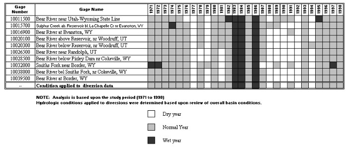
Table 3. Summary of average Dry, Normal, and Wet Year Streamflow at USGS Gaging Stations
| USGS Gage | Gage Name | Hydrologic Condition | JAN | FEB | MAR | APR | MAY | JUN | JUL | AUG | SEP | OCT | NOV | DEC | Total |
| 10011500 | Bear River near UT-WY State Line | Dry Normal Wet |
2440 2743 3490 |
2043 2372 2928 |
2277 2931 3933 |
6495 7026 5895 |
29835 37050 39968 |
23208 54949 90965 |
7595 20000 42370 |
3577 6311 10855 |
2653 5701 9580 |
2895 4495 7183 |
2578 3630 5090 |
2433 3056 4435 |
80123 139083 209983 |
| 10015700 | Sulphur Cr. ab Res.Bl.La Chapelle Cr.Nr.Evanston, WY | Dry Normal Wet |
96 181 135 |
97 218 277 |
468 765 833 |
639 1934 2064 |
644 2539 6925 |
363 936 2586 |
65 257 443 |
34 75 299 |
12 82 237 |
51 129 268 |
102 181 392 |
115 160 277 |
2417 6987 13800 |
| 10015900 | Sulphur Creek below Reservoir near Evanston, WY | Dry Normal Wet |
46 344 368 |
20 422 663 |
635 995 1133 |
1785 2682 2707 |
2792 4854 6620 |
1958 2976 1897 |
1918 1280 1307 |
1410 1559 2230 |
1049 1177 1813 |
191 670 1591 |
130 532 218 |
151 308 1474 |
11613 16290 18739 |
| 10016900 | Bear R. at Evanston, WY | Dry Normal Wet |
2104 4168 6598 |
2085 4225 9306 |
6685 10391 19285 |
13571 21921 26056 |
27361 53606 83172 |
18256 54331 109371 |
3495 14865 27715 |
1556 3051 12344 |
834 3304 11697 |
941 4877 12137 |
1031 4941 9014 |
1384 4373 8525 |
75956 169863 305546 |
| 10020100 | Bear R. ab res. nr Woodruff, URT | Dry Normal Wet |
2235 4675 7157 |
2189 4753 10093 |
6618 11805 20917 |
10311 23201 30450 |
23649 56136 99873 |
17156 55594 129040 |
1753 16253 28523 |
921 2648 13477 |
703 2955 12223 |
8 5517 13163 |
1714 5329 9777 |
1820 4784 9247 |
65535 178020 351753 |
| 10011500 | Bear R. bel res. nr Woodruff, UT | Dry Normal Wet |
1073 3447 5380 |
1020 3544 5070 |
1156 7158 17060 |
3146 20048 28007 |
24891 53673 86843 |
38200 60309 118550 |
5776 22031 32507 |
1610 4371 12770 |
986 4119 10720 |
713 4150 12720 |
685 3578 11997 |
833 3365 7410 |
77858 178700 316907 |
| 10026500 | Bear R. nr Randolph, UT | Dry Normal Wet |
2754 6813 7440 |
2491 7466 10970 |
3976 16963 25900 |
3553 28230 40057 |
4671 45971 91273 |
15145 45408 118957 |
6144 22712 40397 |
2015 8299 18237 |
1212 5639 15613 |
1905 7878 18183 |
2678 7925 17330 |
2634 6901 10410 |
41960 187501 368843 |
| 10028500 | Bear R. bel Pixley Dam, near Cokeville, WY | Dry Normal Wet |
1972 4745 6098 |
1665 4836 7736 |
3744 11520 20226 |
3934 18627 32192 |
1693 40023 73447 |
7601 38213 81000 |
6842 25526 40990 |
2572 9038 20293 |
1492 5950 18027 |
1735 6162 15040 |
2255 5932 13319 |
1959 5260 8975 |
31514 158477 300008 |
| 10032000 | Smiths Fork nr Border, WY | Dry Normal Wet |
3606 3671 5009 |
3243 3237 4450 |
3847 3669 8638 |
8503 9074 12126 |
16611 34070 49692 |
13589 39604 64272 |
6937 20052 29466 |
5109 10016 13370 |
4162 6728 8624 |
4226 5648 7667 |
3706 4668 6148 |
3366 4172 5258 |
65606 130121 195645 |
| 10038000 | Bear R. bel Smiths Fork, nr Cokeville, WY | Dry Normal Wet |
8301 13649 17153 |
7510 13859 20767 |
12018 28008 48313 |
14142 52402 74707 |
21507 88566 150067 |
26874 92123 201367 |
15875 50178 81780 |
7679 19419 39187 |
6429 14348 34513 |
6998 16943 36877 |
8477 16393 33080 |
7884 14929 5258 |
120335 372552 667853 |
| 10038000 | Bear R. at Border, WY | Dry Normal Wet |
8348 14320 18950 |
7587 14374 22400 |
12348 28460 51690 |
13549 55596 75760 |
18140 89113 145567 |
22467 91543 206667 |
14131 50541 81847 |
6274 19337 37510 |
5638 13898 32103 |
6792 17291 34320 |
8400 16919 32543 |
8060 15260 24390 |
108481 377182 672493 |
User Notes:The Gaging Data Table presents the average historic gaging data for each hydrologic condition used in the model. Only the data pertaining to the hydrologic condition being modeled are included in each respective model. These data represent the discharge which can be expected to occur each month in an average dry, normal, or wet year at all the gages used in the model.
2.2.3 Diversion Data
The Bear River Commission publishes diversion records in each of its Biennial Reports. These records were compiled to form the basis of diversion data input to the model. A complete record of diversions exists for the entire basin for the study period of 1971 through 1998. Provisional diversion data reflecting recent years (1996 through 1998) were obtained from the Wyoming State Engineers Office and directly from the Bear River Commission. Following completion of the model, the Bear River Commission published the 1997-1998 Biennial Report which included finalized diversion data for that period. These data were compared to the provisional data and no significant differences were observed.
Estimates of monthly diversions at each of 36 key specific diversions (see Appendix E) were computed for each of the three hydrologic conditions based upon the annual condition presented in Table 2. Key diversions were defined as those locations where greater than 10 cfs are diverted from the river. Eight aggregated diversions for all other diversions in Wyoming were added to complete the water balance for the basin (Appendix F). Diversions within Utah and Idaho were aggregated and modeled as single nodes. All diversions that are specified in the Bear River Compact are included, either explicitly in the model or in the Results Worksheets as data inputs (Table 4).
Table 4. Summary of Average Dry, Normal, and Wet Year Diversion Data
| Node | Diversion Name | Condition | JAN | FEB | MAR | APR | MAY | JUN | JUL | AUG | SEP | OCT | NOV | DEC |
| Node 1.01 | Lannon & Lone Mountain | Dry Normal Wet |
0 0 0 |
0 0 0 |
0 0 0 |
0 0 0 |
886 633 419 |
1010 1087 918 |
554 922 893 |
115 450 476 |
85 502 348 |
0 0 0 |
0 0 0 |
0 0 0 |
| Node 1.02 | Hillard West Side | Dry Normal Wet |
0 0 0 |
0 0 0 |
0 0 0 |
0 0 0 |
975 244 383 |
1720 1467 1054 |
911 1698 1161 |
201 393 812 |
184 701 439 |
0 0 0 |
0 0 0 |
0 0 0 |
| Node 1.03 | Bear Canal | Dry Normal Wet |
0 0 0 |
0 0 0 |
0 0 0 |
0 0 0 |
2071 565 525 |
3456 3712 2044 |
1886 3112 3560 |
551 715 1161 |
348 1068 1142 |
0 0 0 |
0 0 0 |
0 0 0 |
| Node 1.04 | Crown & Pine Grove | Dry Normal Wet |
0 0 0 |
0 0 0 |
0 0 0 |
0 0 0 |
770 438 463 |
1479 1571 1675 |
725 1375 1524 |
207 605 673 |
181 456 196 |
0 0 0 |
0 0 0 |
0 0 0 |
| Node 1.05 | McGraw & Big Bend | Dry Normal Wet |
0 0 0 |
0 0 0 |
0 0 0 |
0 0 0 |
1044 999 305 |
1105 1775 1767 |
422 931 1377 |
200 648 811 |
107 397 756 |
0 0 0 |
0 0 0 |
0 0 0 |
| Node 1.06 | Lewis | Dry Normal Wet |
0 0 0 |
0 0 0 |
0 0 0 |
0 0 0 |
152 92 161 |
333 354 353 |
370 442 414 |
116 287 355 |
37 139 182 |
0 0 0 |
0 0 0 |
0 0 0 |
| Node 1.07 | Meyers No. 2 | Dry Normal Wet |
0 0 0 |
0 0 0 |
0 0 0 |
0 0 0 |
90 35 15 |
277 185 91 |
373 363 357 |
184 333 380 |
121 195 169 |
0 0 0 |
0 0 0 |
0 0 0 |
| Node 1.08 | Meyers No. 1 | Dry Normal Wet |
0 0 0 |
0 0 0 |
0 0 0 |
0 0 0 |
170 72 19 |
233 236 30 |
226 310 305 |
168 221 278 |
59 74 73 |
0 0 0 |
0 0 0 |
0 0 0 |
| Node 1.09 | Meyers Irrigation | Dry Normal Wet |
0 0 0 |
0 0 0 |
0 0 0 |
0 0 0 |
230 80 0 |
248 336 143 |
204 297 319 |
121 206 225 |
46 92 28 |
0 0 0 |
0 0 0 |
0 0 0 |
| Node 1.10 | Evanston Pipeline | Average Year |
0 |
0 |
0 |
0 |
342 |
519 |
719 |
652 |
464 |
0 |
0 |
0 |
| Node 1.11 | Booth | Dry Normal Wet |
0 0 0 |
0 0 0 |
0 0 0 |
0 0 0 |
437 297 202 |
757 745 693 |
502 766 951 |
335 557 567 |
169 404 407 |
0 0 0 |
0 0 0 |
0 0 0 |
| Node 1.12 | Anel | Dry Normal Wet |
0 0 0 |
0 0 0 |
0 0 0 |
0 0 0 |
226 229 153 |
336 737 235 |
208 347 405 |
57 162 77 |
21 136 202 |
0 0 0 |
0 0 0 |
0 0 0 |
| Node 1.13 | Evanston Water Supply | Dry Normal Wet |
0 0 0 |
0 0 0 |
0 0 0 |
0 0 0 |
141 77 64 |
282 372 87 |
257 409 130 |
181 317 165 |
57 166 106 |
0 0 0 |
0 0 0 |
0 0 0 |
| Node 3.01 | Evanston Water Ditch | Dry Normal Wet |
0 0 0 |
0 0 0 |
0 0 0 |
0 0 0 |
616 213 0 |
1197 1165 356 |
895 1077 848 |
603 884 560 |
336 351 118 |
0 0 0 |
0 0 0 |
0 0 0 |
| Node 3.02 | Rocky Mtn & Blyth | Dry Normal Wet |
0 0 0 |
0 0 0 |
0 0 0 |
0 0 0 |
474 505 102 |
600 836 484 |
344 554 886 |
214 296 762 |
170 288 499 |
0 0 0 |
0 0 0 |
0 0 0 |
| Node 4.01 | John Simms | Dry Normal Wet |
0 0 0 |
0 0 0 |
0 0 0 |
0 0 0 |
627 599 353 |
616 990 695 |
428 546 483 |
298 478 507 |
193 451 352 |
0 0 0 |
0 0 0 |
0 0 0 |
| Node 4.02 | S P Ramesy | Dry Normal Wet |
0 0 0 |
0 0 0 |
0 0 0 |
0 0 0 |
635 465 229 |
747 1127 686 |
311 662 759 |
227 406 194 |
116 430 142 |
0 0 0 |
0 0 0 |
0 0 0 |
| Node 5.01 | Chapman Canal | Dry Normal Wet |
0 0 0 |
0 0 0 |
0 0 0 |
0 0 0 |
5825 5209 2965 |
5838 8040 3247 |
1937 4187 2532 |
612 1595 642 |
383 1402 417 |
0 0 0 |
0 0 0 |
0 0 0 |
| Node 5.02 | Morris Bros (Lower) | Dry Normal Wet |
0 0 0 |
0 0 0 |
0 0 0 |
0 0 0 |
143 152 743 |
179 253 793 |
116 87 744 |
52 57 65 |
80 59 72 |
0 0 0 |
0 0 0 |
0 0 0 |
| Node 5.04 | Tunnel | Dry Normal Wet |
0 0 0 |
0 0 0 |
0 0 0 |
0 0 0 |
575 557 245 |
1173 1602 1581 |
376 552 559 |
120 216 210 |
81 194 259 |
0 0 0 |
0 0 0 |
0 0 0 |
| Node 6.01 | Woodruff Narrows | Dry Normal Wet |
0 0 0 |
0 0 0 |
0 0 0 |
0 0 0 |
34757 34351 62273 |
11242 26750 58430 |
7608 21457 53250 |
6697 19138 51947 |
5940 17901 54207 |
0 0 0 |
0 0 0 |
0 0 0 |
| Node 7.01 | Francis Lee | Dry Normal Wet |
0 0 0 |
0 0 0 |
0 0 0 |
0 0 0 |
1923 1524 1091 |
2797 2999 2831 |
555 1484 1236 |
168 544 37 |
97 436 301 |
0 0 0 |
0 0 0 |
0 0 0 |
| Node 7.02 | Bear River Canal | Dry Normal Wet |
0 0 0 |
0 0 0 |
0 0 0 |
0 0 0 |
2922 2424 1851 |
3797 4872 3991 |
752 1803 1802 |
134 295 262 |
100 487 150 |
0 0 0 |
0 0 0 |
0 0 0 |
| Node 7.03 | Total Lower Utah | Dry Normal Wet |
0 0 0 |
0 0 0 |
0 0 0 |
0 0 0 |
30744 34210 25661 |
54918 60344 65985 |
11019 27279 23764 |
3291 3794 1708 |
2604 5317 1572 |
0 0 0 |
0 0 0 |
0 0 0 |
| Node 8.01 | Pixley Diversions | Dry Normal Wet |
0 0 0 |
0 0 0 |
0 0 0 |
0 0 0 |
2276 2464 5224 |
3466 4003 6427 |
925 913 639 |
46 24 79 |
95 151 18 |
0 0 0 |
0 0 0 |
0 0 0 |
| Node 8.02 | BQ Diversion | Dry Normal Wet |
0 0 0 |
0 0 0 |
0 0 0 |
0 0 0 |
3325 2612 6014 |
7815 6924 10403 |
1625 2411 1721 |
77 123 194 |
22 11 0 |
0 0 0 |
0 0 0 |
0 0 0 |
| Node 10.02 | Button Flat | Dry Normal Wet |
0 0 0 |
0 0 0 |
0 0 0 |
0 0 0 |
44 89 0 |
160 186 245 |
162 236 63 |
50 172 22 |
0 71 17 |
0 0 0 |
0 0 0 |
0 0 0 |
| Node 10.03 | Emelle | Dry Normal Wet |
0 0 0 |
0 0 0 |
0 0 0 |
0 0 0 |
186 116 0 |
816 842 404 |
675 817 761 |
242 606 491 |
28 54 42 |
0 0 0 |
0 0 0 |
0 0 0 |
| Node 10.04 | Cooper | Dry Normal Wet |
0 0 0 |
0 0 0 |
0 0 0 |
0 0 0 |
335 277 530 |
462 472 1038 |
284 295 29 |
114 73 5 |
0 26 0 |
0 0 0 |
0 0 0 |
0 0 0 |
| Node 10.05 | Covey | Dry Normal Wet |
0 0 0 |
0 0 0 |
0 0 0 |
0 0 0 |
2878 2518 2292 |
3745 5914 4594 |
2327 5306 4166 |
973 3122 3189 |
423 1236 1443 |
0 0 0 |
0 0 0 |
0 0 0 |
| Node 10.06 | VH Canal | Dry Normal Wet |
0 0 0 |
0 0 0 |
0 0 0 |
0 0 0 |
314 425 385 |
569 689 865 |
484 660 723 |
435 654 906 |
172 491 427 |
0 0 0 |
0 0 0 |
0 0 0 |
| Node 10.07 | Goodell | Dry Normal Wet |
0 0 0 |
0 0 0 |
0 0 0 |
0 0 0 |
196 238 26 |
360 418 195 |
384 478 309 |
278 416 266 |
171 329 68 |
0 0 0 |
0 0 0 |
0 0 0 |
| Node 10.08 | Whites Water | Dry Normal Wet |
0 0 0 |
0 0 0 |
0 0 0 |
0 0 0 |
729 830 1118 |
1095 1885 2078 |
836 1427 1941 |
454 1215 1251 |
243 520 534 |
0 0 0 |
0 0 0 |
0 0 0 |
| Node 10.09 | S Branch Irrigation | Dry Normal Wet |
0 0 0 |
0 0 0 |
0 0 0 |
0 0 0 |
1017 854 1811 |
940 1213 3790 |
457 645 1938 |
95 592 568 |
38 242 107 |
0 0 0 |
0 0 0 |
0 0 0 |
| Node 11.02 | Alonzo F. Sights | Dry Normal Wet |
0 0 0 |
0 0 0 |
0 0 0 |
0 0 0 |
400 647 656 |
746 1238 3592 |
524 770 582 |
234 325 184 |
27 98 0 |
0 0 0 |
0 0 0 |
0 0 0 |
| Node 11.03 | Oscar E. Snyder | Dry Normal Wet |
0 0 0 |
0 0 0 |
0 0 0 |
0 0 0 |
461 654 1054 |
942 1593 3275 |
588 1196 1214 |
381 347 356 |
260 298 286 |
0 0 0 |
0 0 0 |
0 0 0 |
| Node 11.04 | Cook Brothers | Dry Normal Wet |
0 0 0 |
0 0 0 |
0 0 0 |
0 0 0 |
1906 1247 1531 |
2084 3135 4163 |
1141 1514 1041 |
1323 1060 274 |
796 1391 455 |
0 0 0 |
0 0 0 |
0 0 0 |
| Node 12.02 | Total Idaho | Dry Normal Wet |
0 0 0 |
0 0 0 |
0 0 0 |
0 0 0 |
16439 14094 11487 |
18876 27139 28680 |
10008 14848 13788 |
5570 7282 7071 |
5224 6947 5008 |
0 0 0 |
0 0 0 |
0 0 0 |
| Node 12.03 | Rainbow | Dry Normal Wet |
6943 11163 16672 |
6552 11530 20510 |
15002 27234 53741 |
14541 52840 89788 |
8640 82646 174526 |
3435 67552 197474 |
3663 39806 76965 |
1478 16195 39597 |
1444 11167 35047 |
2793 15798 36646 |
5329 15436 34007 |
4903 13133 21810 |
| Node 12.04 | Stewart Dam | Dry Normal Wet |
581 299 188 |
644 291 201 |
624 485 495 |
451 378 430 |
490 646 1084 |
666 2506 17187 |
663 1004 13762 |
796 691 640 |
706 949 742 |
721 659 511 |
407 513 384 |
309 422 314 |
| The following diversions are not modeled explicitely in the Bear River Model. They are included in the evaluation of Compact Allocations and Water Emergencies. | ||||||||||||||
| Hilliard East Side | Dry Normal Wet |
0 0 0 |
0 0 0 |
0 0 0 |
0 0 0 |
296 34 0 |
1238 534 77 |
1122 1462 1226 |
32 417 520 |
87 477 412 |
0 0 0 |
0 0 0 |
0 0 0 | |
| Quinn Bourne | Dry Normal Wet |
0 0 0 |
0 0 0 |
0 0 0 |
0 0 0 |
311 237 178 |
340 446 580 |
168 398 722 |
57 216 467 |
14 75 50 |
0 0 0 |
0 0 0 |
0 0 0 | |
| Upper Utah =sum Hatch + Hovarka |
Dry Normal Wet |
0 0 0 |
0 0 0 |
0 0 0 |
0 0 0 |
413 249 105 |
908 1062 858 |
542 823 988 |
262 462 654 |
91 132 376 |
0 0 0 |
0 0 0 |
0 0 0 | |
Engineering Notes:2.2.4 Import and Export DataThe following sections summarize the sources of data for each division.
Upper Utah Section - Upper Division
- 1971-1998 data were obtained from tables published in the Bear River Commission Reports. Note that diversion records for the Hatch diversion began in 1992. These diversions are not explicitly modeled; however, their annual average totals are included in the Compact Allocation Worksheet in the results.
Wyoming Section - Upper Division
- 1971-1996 data were obtained from tables published in the Bear River Commission Reports.
- 1997-1998 data were obtained from preliminary diversion records provided by Jade Henderson, State Engineer's Cokeville Office. At the time that these data were provided, there was not yet a published Biennial Report for the period. In late April, 2000, the Bear River Commission published the 1997-1998 Biennial Report. Diversion records from these reports were spot checked against the preliminary data. This check resulted in no significant changes between the preliminary data and the published data.
Lower Utah Section - Upper Division
- 1971-1996 data were obtained from tables published in the Bear River Commission Reports.
- 1997-1999 date were obtained from preliminary diversion records provided by Don Barnett, Bear River Commission Office. At the time that these data were provide, Biennial Reports were not yet available for this period. In late April, 2000, the Bear River Commission published the 1997-1998 Biennial Report. Diversion records from these reports were spot checked against the preliminary data. This check resulted in no significant changes between the preliminary data and the published data.
Wyoming Section - Lower Division
- 1971-1996 data were obtained from tables published in the Bear River Commission Reports.
- 1997-1998 data were obtained from preliminary diversion records provided by Jade Henderson, State Engineer's Cokeville Office. At the time that these data were provided, there was not yet a published Biennial Report for the period. In late April, 2000, the Bear River Commission published the 1997-1998 Biennial Report. Diversion records from these reports were spot checked against the preliminary data. This check resulted in no significant changes between the preliminary data and the published data.
Wyoming Section - Central Division
- 1971-1996 date were obtained from tables published in the Bear River Commission Reports.
- 1997-1999 data were obtained from preliminary diversion records provided by Jade Henderson, State Engineer's Cokeville Office. At the time that these data were provided, Biennial Reports for this period were not yet available. In late April, 2000, the Bear River Commission published the 1997-1998 Biennial Report. Diversion records from these reports were spot checked against the preliminary data. This check resulted in no significant changes between the preliminary data and the published data.
Idaho Section - Central Division
- 1971-1996 data were obtained from tables published in the Bear River Commission Reports.
- 1997-1999 data were obtained from preliminary diversion records provided by Don Barnett, Bear River Commission Office. At the time that these data were provided, Biennial Reports for this period were not yet available. In late April, 2000, the Bear River Commission published the 1997-1998 Biennial Report. Diversion records from these reports were spot checked against the preliminary data. This check resulted in no significant changes between the preliminary data and the published data.
Bear River below Stewart Dam
- 1970-1999 data were provided by the PacifiCorp Office in Salt Lake City. The data were provided by Scott Johnson from that office. Records for the flow in the Bear River below Stewart Dam are published in the Bear River Commission Biennial Report only for the summer months. Since year-round data at this location was required for the model, PacifiCorp was contacted in order to obtain winter data at this gage. Although the summer records published in the Biennial Report varied slightly from those records provided by PacifiCorp, PacifiCorp's numbers for both summer and winter flows were used to keep consistency in the data source.
Rainbow Inlet
- 1971-1998 Data is from tables published in the Bear River Commission Reports.
Based upon the determination of hydrologic condition at each USGS gaging station conducted during Task 3A of the Bear River Planning Study, overall basin conditions were estimated (Table 2). Examination of Table 2 reveals that in general, the hydrologic conditions were very consistent throughout the basin. A row summarizing basin-wide hydrologic conditions for the Bear River Basin appears at the bottom of the table. From this selection of hydrologic year type, average monthly diversions for each of the three hydrologic conditions were determined.
Average monthly diversion data were computed based upon the basin-wide conditions (Appendix E). Average dry year diversions represent the average of diversions recorded during the six dry years (1977, 1979, 1988, 1990, 1992, and 1994), average normal year diversions represent the average of diversions during the nineteen normal years (1971-1976, 1978, 1980-1982, 1985, 1987, 1989, 1991, 1993, and 1995-1998), and average wet year diversions represent the average of diversions during the three wet years (1983, 1984, and 1986).
User Notes:
This worksheet provides a summary of the diversions which can be expected to occur at each node during a typical dry, normal, or wet year. This worksheet is a means of providing input data to the model; there are no computations conducted within it. Note that all nodes are listed in the table, even if no diversions occur at them. At the top of the worksheet are buttons which also take the User to a table summarizing the total monthly diversions in each reach.
The Broadbent Supply Ditch imports water from the Green River Basin. In 1999, it was fitted with a recorder and telemetry system which improved the ability to document this import. According to the 1999 Biennial Report, 24.8 acre-feet were imported for the period July 31 to the end of September.
Engineering Notes:2.3 The Computation WorksheetsAverage monthly historic data are lacking for the Broadbent Ditch because it was only recently equipped with gaging equipment. Based upon the 1999 Biennial Report, 24.8 acre- feet were imported over a 62 day period. This converts to an average of 0.2 cfs or an average of approximately 12 acre-feet per month. This value was used as the average monthly import for the Broadbent Ditch during the irrigation season in each hydrologic condition.
User Notes:
The Imports / Exports Table summarizes the monthly imports to or exports from other basins. In the Bear River Model, the only imports incorporated are those associated with the Broadbent Supply Ditch. There are no basin exports incorporated herein, although that capability exists at all nodes.
The spreadsheet model determines the water budget at node points along the river, reflecting inflows from gaged and ungaged tributaries and diversions from delivery points. The historic or estimated river headgate diversions are the demands that drive the model. The consumptive use portion of these diversions must be estimated along with the return flows. These return flows eventually return to the stream system and are available for future diversions.
2.3.1 Return Flows
The unused portion of a headgate diversion either returns to the river as surface runoff during the month it is diverted, or "deep percolates" into the alluvial aquifer. The deep percolation portion returns to the river through the aquifer but generally lags the time of diversion by several months, or even years. It is important for the model to simulate both the percent of headgate diversions that return to the river, and the timing of which this unused portion returns. In the Bear River Basin, water from the river is reused many times from the headwaters to the Great Salt Lake.
Diversion efficiency is the common measure of the portion of headgate diversion that is consumed, and therefore not returned to the river. Diversion efficiency for municipal and industrial use is the percent of headgate diversion that makes it to the treatment plant or industrial site. The remaining percent is lost during conveyance, and returns to the river as surface runoff or deep percolation. Diversions for agricultural use experience both conveyance losses and application losses, and both these loss percentages return to the river as surface runoff or deep percolation. Additional discussion of the consumptive use analysis and return flow study is contained in Tasks 2A, 2B, and 2C Memorandum, Bear River Planning Study.
Engineering Notes:2.3.2 Return Options TablesTable 5 shows the conveyance efficiencies estimated for the key ditch systems represented in the modeling effort for the upper division. The upper division aggregate ditch systems were assigned a conveyance efficiency of 65 percent, because they represent smaller ditches generally irrigating lands close to the river. Table 6 shows the conveyance efficiencies estimated for the key ditch systems represented in the modeling effort for the central division. The central division aggregate ditch systems were assigned a conveyance efficiency of 65 percent, again because they represent smaller ditches generally irrigating lands close to the river.
In addition to conveyance efficiencies, Table 5 shows the suggested application efficiency for the key ditch systems in the upper division. Because lands in the upper division are flood irrigated, the application efficiencies are all 55 percent. An application efficiency of 55 percent is also used for aggregated ditch systems. Table 6 shows the suggested application efficiency for the key ditch systems in the central division. An application efficiency of 65 percent was used for aggregated ditch systems in the central division, which represents an average of key ditch system efficiencies.
The model uses a diversion efficiency that represents the actual amount of headgate diversion used to satisfy crop consumptive use demands. It is calculated as the product of conveyance efficiency and application efficiency. The diversion efficiency is also provided in Tables 5 and 6.
Table 5. Upper Division Diversion Efficiencies
Model Node ID Diversion Name Converance Efficiency Application Efficiency Diversion Efficiency Irrigation Methods 1.14 Hilliard East Fork 40% 55% 22% 100% Flood 1.01 Lannon and Lone Mountain 45% 55% 25% 100% Flood 1.02 Hilliard West Side 40% 55% 22% 100% Flood 1.03 Bear Canal 40% 55% 22% 100% Flood 1.04 Crown and Pine Grove 50% 55% 27% 100% Flood 1.05 McGraw (and Big Ben) 55% 55% 30% 100% Flood 1.06 Lewis 55% 55% 30% 100% Flood 1.07 Myers No 2 50% 55% 27% 100% Flood 1.08 Myers No 1 50% 55% 27% 100% Flood 1.09 Myers Irrigation 55% 55% 30% 100% Flood 1.11 Booth 50% 55% 27% 100% Flood 1.12 Anel 55% 55% 30% 100% Flood 1.13 Evanston Water Supply 50% 55% 27% 100% Flood 3.01 Evanston Water Ditch 65% 55% 36% 100% Flood 3.02 Rocky Mountain Blythe 65% 55% 36% 100% Flood 4.01 John Simms 65% 55% 36% 100% Flood 4.02 SP Ramsey 60% 55% 33% 100% Flood 5.01 Chapman (Wyoming portion) 50% 55% 27% 100% Flood 5.02 Morris Brothers 65% 55% 36% 100% Flood 5.03 Tunnel 65% 55% 36% 100% Flood 7.01 Francis Lee 60% 55% 33% 100% Flood 7.02 Bear River Canal 60% 55% 33% 100% Flood Varies Aggregate Systems 65% 55% 36% 100% Flood
Table 6. Central Division Diversion Efficiencies
Model Node ID Diversion Name Converance Efficiency Application Efficiency Diversion Efficiency Irrigation Methods 7.03 Utah Aggregate Ditches 45% 65% 30% 67% Flood 33% Center Pivot Sprinkler 8.01 Pixley Dam 55% 60% 33% 90% Flood 10% Center Pivot Sprinkler 10.02 Button Flax 65% 55% 36% 100% Flood 10.03 Emelle 65% 55% 36% 100% Flood 10.04 Cooper 65% 55% 36% 100% Flood 10.05 Covey 45% 65% 30% 70% Flood 30% Center Pivot Sprinkler 10.06 VH Canal 55% 85% 47% 100% Center Pivot Sprinkler 10.07 Goodell 55% 85% 47% 100% Center Pivot Sprinkler 10.08 Whites Water 60% 65% 40% 60% Flood 40% Center Pivot Sprinkler 10.09 S. Branch Irrigation 60% 70% 42% 40% Flood 60% Center Pivot Sprinkler 11.01 Alonzo F. Sights 65% 65% 42% 60% Flood 40% Center Pivot Sprinkler 11.02 Oscar E. Snyder 65% 55% 36% 100% Flood 11.03 Cook Brothers 65% 55% 36% 100% Flood Varies Aggregates Systems 65% 65% 42% 67% Flood 33% Center Pivot Sprinkler
User Notes:
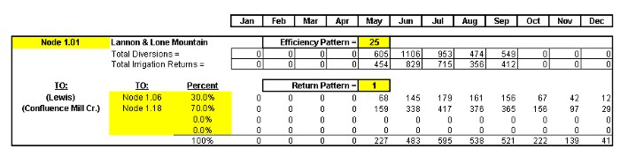
This worksheet computes the return flows from irrigation diversions, mainly. For every node, the return flow is computed based upon estimates of consumptive use associated with the crops irrigated, the extent and location of the irrigated acreage, and canal losses. For clarification, all cells which can be modified by the User are highlighted in yellow. The features of this worksheet are discussed in the following sections. Figure 6 displays an example table from the Return Flows worksheet.
Figure 6. Example Return Flows Node TableTotal Diversions
These values are retrieved automatically from the Diversion Data tables.
Efficiency Pattern
The model applies one of 17 pre-determined irrigation efficiency patterns to the water diverted at each node. The efficiency patterns represent that portion of the diversion which is lost to the system as a consumption. The remainder are losses, e.g., conveyance and on-farm efficiency losses (e.g., flood vs sprinkler irrigation efficiency), which are returned to the system at other river points. For example, an efficiency pattern of 25 means that 75% of the water diverted eventually returns to the river either by surface or subsurface flow and that 25% is consumed. These patterns are included on the Options Tables worksheet of the model. By entering the number associated with a pattern in this cell, the efficiency pattern is applied.
Total Irrigation Returns
These data are computed by multiplying the Total Diversions by the selected Efficiency Pattern. For example, if a month shows a Total Diversion of 883 acre-feet and an Efficiency Pattern of 25 is selected, the Total Irrigation Returns from that diversion will be 662 acre-feet (883 x (1.0-.25) = 662) distributed in a temporal pattern as specified by the Return Pattern. It is assumed that there is not sufficient variation in the monthly efficiency to justify a monthly- varying pattern.
TO and Percent
This feature allows the User to define the node in the model where irrigation returns will return. Return locations were determined based upon field inspection, local knowledge, and/or aerial photographs. By entering the node number in the TO box, and the relative percentage of the Total Irrigation Returns that are expected to return to that node, the Total Irrigation Returns are distributed accordingly. Note that the percentages entered at each node must total 100% or an error message will appear warning the User that all returns have not been accounted.
Return Pattern
The Return Pattern feature allows the User to select between four different temporal patterns representing the lagged time effect of irrigation returns to the river. The four Return Patterns available are displayed in the Irrigation Return Lags section of the Options Table. Not all of the water diverted at a node returns to the river in the same month. The lags between the month in which a diversion occurs and the month the irrigation returns actually arrive in the river are estimated.
The Return Pattern feature first directs the model to account for that portion of irrigation returns occurring in the same month as the diversion. It then directs the model to add returns lagged from previous months. In this model, it was assumed that all irrigation returns will occur during the month it is diverted and within three additional months.
Irrigation Returns: Node Totals Table
This table collects all of the irrigation returns that have been sent to each Node and provides their sum. It is accessed via the "View 'Node Totals' Summary Table" button located at the top of the worksheet.
Irrigation Returns: Reach Totals Table
This table collects all of the irrigation returns that have been sent to each Reach and provides their sum. It is accessed via the "View 'Reach Totals' Summary Table" button located at the top of the worksheet.
These tables store the patterns specified in the Return Flow worksheet apart from the node by node calculations. They are stored in a separate worksheet than the Return Flows.
Engineering Notes:2.3.3 Evaporative LossesThe unused, or inefficient, portion of diversions are returned to the river either by direct surface runoff, or through the alluvial aquifer. For modeling purposes, an estimate must be made of both:
- the location or locations on the river where the unused portion of diversions will return, and
- the timing of those returns.
The irrigated acreage GIS theme was used to estimate these locations, shown in Table 7 for the upper division and Table 8 for the central division. In addition to the return flow node location in the river, Tables 7 and 8 show the return flow pattern used to represent each ditch system. Additional discussion of the return flow analysis is contained in Tasks 2A, 2B, and 2C Memorandum, Bear River Planning Study.
Table 7. Upper Division Return Flow Locations and Patterns
Model Node ID Diversion Name Return Nodes Return Pattern 1.14 Hilliard East Fork 100% Ag-Sulphur Creek bl Reservoir 1 1.01 Lannon and Lone Mountain 30% Lewis Ditch 70% Confluence with Mill Ck 2 1.02 Hilliard West Side 100% Sulphur Creek Reservoir 1 1.03 Bear Canal 60% Sulphur Creek Reservoir 40% Ag-Sulphur Creek bl Reservoir 1 1.04 Crown and Pine Grove 25% Lewis 25% Cnfluence with Mill Ck 50% Myers No 2 2 1.05 McGraw (and Big Ben) 100% Lewis 2 1.06 Lewis 100% Myers No 1 2 1.07 Myers No 2 100% Myers No 1 2 1.08 Myers No 1 50% Booth 50% Ag-Sulphur Creek bl Reservoir 2 1.09 Myers Irrigation 100% Anel 2 1.11 Booth 100% Evanston Water Ditch 2 1.12 Anel 100% between Mill Creek and Sulphur Creek 2 1.13 Evanston Water Supply 50% Rocky Mountain Blythe 50% John Simms 2 1.15 Ag-Bear River Between Mill Creek and Su 100% Confulence Bear and Sulphur Creek 2 2.04 Ag-Sulphur Creek Above Resevoir 100% Sulphur Creek Res. 2 2.03 Ag-Sulphur Below Reservoir 100% Confulence Bear and Sulphur Creek 2 3.01 Evanston Water Ditch 100% Rocky Mountain Blythe 2 3.02 Rocky Mountain Blythe 70% John Simms 30% SP Ramsey 2 4.01 John Simms 50% SP Ramsey 50% Ag-Bear River between Sulphur and Yellow Creeks 2 4.02 SP Ramsey (also called Adin Brown) 50% Ag-Bear River between Sulphur and Yellow Creeks 50% Chapman 2 4.03 Ag-Bear River between Sulphur and Yello 100% Chapman 2 5.01 Chapman 100% Woodruff Narrows (WY) 2 5.02 Morris Brothers 30% Ag-Bear River between Yellow Creek and Woodruff 70% Woodruff Narrows 2 5.04 Ag-Bear River Yellow Creek and 100% Tunnel 2 5.03 Tunnel 100% Woodruff Narrows 2 7.01 Francis Lee 100% Ag-Utah Diversions 1 7.02 Bear River Canal 100% Ag-Utah Diversions 1
Table 8. Central Division Return Flow Locations and Patterns
Model Node ID Diversion Name Return Node Return Pattern 7.03 Ag-Utah diversion 25% Node 7.04 70%USGS 26500 5% Pixley 2 8.01 Pixley Dam 100% Confluence with Smiths Fork 2 8.02 Ah-Bear river betweenTwin Fork and Smiths Fork 100% Confluence with Smiths Fork 2 10.01 Quinn Bourne 100% Button Flax 2 10.02 Button Flax 100% Emelle 2 10.03 Emelle 50% Cooper Ditch 50% Covey 2 10.04 Cooper 100% Covey 2 10.05 Covey 10% Whites Water 90% Confluence Bear and Smiths Fork 1 10.06 VH Canal 100% Whites Water 1 10.07 Goodell 100% Whites Water 1 10.08 Whites Water 100% Ag-Bear River below Smiths Fork 2 10.09 S. Branch Irrigation 100% Ag-Bear River below Smiths Fork 2 10.10 Ag-Smiths Fork 100% Ag-Bear River below Smiths Fork 2 11.01 Alonzo F. Sights 50% Oscar E. Snyder 50% Cook Brothers 2 11.02 Oscar E. Snyder 50% Cook Brothers 50% Bear River at Border Gage (1003950) 2 11.03 Cook Brothers 50% Bear River at Border Gage 50% Ag-Idaho Diversions 2
User Notes:
The Options Tables incorporate the information used in the computation of irrigation return flow quantities and their timing. The data in the first table, "Irrigation Return Patterns", consist of the percentages of water diverted which eventually will return to the river and be made available to downstream users. The values entered under "Pattern Type" are the amounts of water consumed or lost from the system.
The second worksheet table, "Irrigation Return Lags", controls the timing of these returns. Flows diverted in any month can be lagged up to three months beyond the month in which they are diverted. For example, Return Pattern No. 1 is as follows:
Month 0 1 2 3 Percent 50 15 25 10 For a diversion occurring in June, 50 percent of the Total Irrigation Returns (i.e., that portion not lost to consumptive use, evaporation, etc.) will return in June, 15 percent will return in July, 25 percent will return in August, and the remaining 10 percent will return in September.
Evaporation losses occur from any free water surface in the Bear River Basin, however, in this model development the only calculated evaporation occurs at the two main reservoirs in the system; Sulphur Creek and Woodruff Narrows Reservoirs. Evaporative losses from the river surface are accounted for in the reach gain/loss calculations. Similarly, evaporation losses from Stewart Dam are accounted for in the reach gain/loss calculation for that reach.
In the Bear River Model, two reservoirs were modeled: Sulphur Creek Reservoir located on Sulphur Creek (Node 2.02), and Woodruff Narrows Reservoir located on the mainstem of the Bear River (Node 6.01). Pixley Dam (Node 8.01) and Stewart Dam (Node 12.04) are included in the model as node points only; no storage is allowed at the sites, nor evaporation losses calculated. Evaporation losses are included in the mass balance calculations at each reservoir node.
Engineering Notes:2.3.4 Node TablesPan evaporation data for the Green River, Wyoming, weather station were obtained through the High Plains Climate Center located in Lincoln, NE. No pan evaporation data were available within the Bear River Basin. Because of its proximity to the Bear River Basin, the Green River weather station was assumed to be representative of the basin. The pan evaporation data were adjusted by a factor of 0.6 to estimate evaporation from reservoirs and lakes. Precipitation data for the Evanston, Wyoming weather station were obtained through the Water Resources Data System (WRDS). Using average monthly pan evaporation data and mean monthly precipitation data, the net monthly reservoir evaporation estimates were computed and input to the model. The average annual net evaporation rate was 33.25 inches per acre (Table 9).
Table 9. Summary of Net Evaporation Calculations
Mean Monthly Data (Green River, WY) Jan Feb Mar Aprl May Jun Jul Aug Sep Oct Nov Dec Total Average Monthly Gross Pan Evaporation (inches) 2.53 2.44 2.67 3.24 4.27 5.73 6.29 5.61 4.09 2.83 2.26 2.63 44.6 Average Monthly Precipitation (inches) 1.11 1.03 0.94 0.92 1.16 1.20 1.05 0.89 0.75 0.79 0.69 0.83 11.3 Average Net Evaporation (inches) 1.42 1.41 1.73 2.32 3.12 4.53 5.24 4.72 3.34 2.04 1.57 1.80 33.2
User Notes:
Monthly gross evaporation (inches) and total precipitation (inches) data are included in the table. Pan evaporation data must be adjusted to represent lake surface evaporation prior to entry. The worksheet then computes the net evaporation in inches and applies this factor to the average annual lake surface area.
Each non-storage node is represented in the spreadsheet by an inflow section, which includes inflow from the upstream node, irrigation returns, ungaged gains, and imports, if applicable; and an outflow section, which includes ungaged losses and diversions, if applicable. The algebraic sum of these flows are then the net outflow from the node. In the case of storage nodes, evaporation is included as a loss and flow can either go to or come from storage. Again, the water balance is done for the node and outflow is calculated. Figure 7 displays the Node 1.01 Table (Lannon and Lone Mountain) as an example.
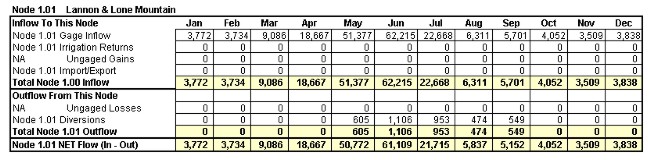
Figure 7. Example Node Table
Engineering Notes:2.3.5 Reach Gain/LossThis is the heart of the spreadsheet model where water budget calculations are performed for each node represented in the basin. Water balance is maintained in a river reach, or at least between reach gain/loss points, by performing the water budget calculations at each node until the outflow from the bottom node in each reach equals the gage flow at that point.
User Notes:
The Node Tables compute the flow available to downstream users (NET flow) using a water budget approach.
NET Flow = Total Node Inflow - Total Node Outflow
where:
Total Node Inflow = Flow from the node located upstream +
Irrigation Returns to this the node +
Ungaged reach gains (if available) +/-
Basin Imports/Exportsand Total Node Outflow = Diversions from the node +
Ungaged LossesThe nodes must be organized in a consecutive order within each reach. Historic diversions at each node are automatically referenced from the Diversion Data worksheet. In the event that the historic demand cannot be met based upon available streamflow, the model will determine the amount that is available and enter that amount. In that event, a warning will be presented to inform the User that a diversion has been shorted.
The Bear River Basin, although of limited geographic size and well-documented by data sources, could not be completely modeled explicitly. Not all water features, such as small tributaries and diversions, are included in the computer representation of the physical system. Therefore, many features are aggregated and modeled, while many others are lumped together between measured flow points in the river by a modeling construct called ungaged reach gains and losses. These ungaged gains and losses account for all water in the budget that is not explicitly named and become a measure of how well the system incorporates physical features.
Engineering Notes:2.4 The Reach/Node WorksheetsUngaged gains to the model include sources such as inflow from un-modeled tributaries, return flows from un-modeled diversions and groundwater inflow. Ungaged losses include factors such as un-modeled diversions, seepage and evaporation from the river. These factors are computed on a reach-by-reach basis using a water budget approach:
Ungaged Gains/Losses = Difference between downstream and upstream gages
+
Total diversions within the Reach -
Total irrigation return flows to the Reach +/-
Reservoir change in storageThe volume of ungaged gains and losses is a good measure of the adequacy of the model and the accuracy of the modeled features. If the volumes are high in comparison to the flow in the river or to diversions, then some major water features have not been modeled or have not been modeled correctly.
User Notes:
The worksheet collects all positive values (Reach Gains) and all negative values (Reach Losses) and creates the two Reach Summary Tables which are viewable with selection of the "Summary" button. Table 10 displays the Ungaged Gains and Losses determined for the Normal Year condition.
Table 10. Summary of Ungaged Reach Gains and Losses for the Normal Hydrologic Conditions
Ungaged Reach Gains
Jan Feb Mar Apr May Jun Jul Aug Sep Oct Nov Dec Reach 1, 2 & 3 1081 1431 6466 12228 15308 7661 2606 0 0 0 357 936 Reach 4 & 5 507 528 1413 1288 6328 8156 4465 554 512 327 291 410 Reach 6 0 0 0 0 0 0 0 0 0 0 0 0 Reach 7 3366 3922 9805 8182 24962 41735 22679 3924 5049 3029 4046 3475 Reach 8 0 0 0 0 0 0 0 0 0 0 0 0 Reach 9 & 10 5233 5786 12819 24717 19196 26146 16230 7019 3837 4611 5551 5445 Reach 11 672 515 451 3194 1186 658 0 0 0 0 33 252 Reach 12 0 0 0 0 3665 0 0 0 1122 0 0 0 Ungaged Reach Loss
Jan Feb Mar Apr May Jun Jul Aug Sep Oct Nov Dec Reach 1, 2 & 3 0 0 0 0 0 0 0 2289 1474 1417 0 0 Reach 4 & 5 0 0 0 0 0 0 0 0 0 0 0 0 Reach 6 0 0 0 0 0 0 0 0 0 0 0 0 Reach 7 0 0 0 0 0 0 0 0 0 0 0 0 Reach 8 2067 2630 5444 9603 14650 25580 14220 7373 3492 2483 2273 1641 Reach 9 & 10 0 0 0 0 0 0 0 0 0 0 0 0 Reach 11 0 0 0 0 0 0 1661 3595 2107 1080 0 0 Reach 12 2859 2553 740 2378 0 4912 3207 492 0 1940 1341 1705
In most cases, the Ungaged Reach Gains and Losses were computed for single reaches which are bound on both the upstream and downstream ends by gages. In those cases where the downstream end of a reach is not a gage, exceptions to this rule occur. These instances are discussed as follows:
A. Reaches 1, 2 and 3 Ungaged Gains and Losses were computed for the combined reaches and distributed between the upstream end of Reach 1 (Bear River) and Reach 2 (Sulphur Creek) in proportion to the ratio of the total annual discharges at the two upstream gages. For this computation, the water budget presented above consisted of the following terms:
Difference in Gaged Flows = Bear River at Evanston, WY (Gage 10016900)
-
Bear River near UT-WY State Line (Gage 10011500)
-
Sulphur Creek above Reservoir below La Chapelle
Creek near Evanston, WY (Gage 10015700)Total Diversions = Total Diversions Reach 1 +
Total Diversions Reach 2 +
Total Diversions Reach 3 +
Change in Reservoir Storage (Sulphur Creek)Total Return Flows = Total Returns Reach 1 +
Total Returns Reach 2 +
Total Returns Reach 3B. Reaches 4 and 5
Ungaged Gains and Losses were computed for the combined reaches. Combined Gains were added to the upstream end of Reach 4 and combined Losses were taken at the downstream end of Reach 5. For this computation, the water budget presented above consisted of the following terms:
Difference in Gaged Flows = Bear River above Reservoir, near Woodruff, UT
(Gage 10020100)
-
Bear River at Evanston, WY (Gage 10016900)Total Diversions = Total Diversions Reach 4 +
Total Diversions Reach 5Total Return Flows = Total Returns Reach 4 +
Total Returns Reach 5C. Reaches 9, 10 and 11 Ungaged Gains and Losses were computed for the combined reaches and distributed between the upstream end of Reach 9 (Bear River) and Reach 10 (Smiths Fork) in proportion to the ratio of the total annual discharges at the two upstream gages. For this computation, the water budget presented above consisted of the following terms:
Difference in Gaged Flows = Bear River below Smiths Fork, near Cokeville, WY
(USGS 10038000)
-
Smiths Fork near Border, WY (USGS 1003200)
-
Bear River below Pixley Dam, near Cokeville, WY
(USGS 10028500)Total Diversions = Total Diversions Reach 9 +
Total Diversions Reach 10 +
Total Diversions Reach 11Total Return Flows = Total Returns Reach 9 +
Total Returns Reach 10 +
Total Returns Reach 11
The following sections present information pertinent to each specific reach in the Bear River Model. Included in these sections are listings, issues and assumptions pertaining to each reach.
2.4.1 Reach 1
Reach 1 consists of the following nodes listed in the order they are placed in the model:
| Node 1.00 | USGS 10011500: Bear River near UT-WY State Line |
| Node 1.01 | Lannon & Lone Mountain |
| Node 1.02 | Hilliard West Side |
| Node 1.03 | Bear Canal |
| Node 1.04 | Crown & Pine Grove |
| Node 1.05 | McGraw & Big Bend |
| Node 1.06 | Lewis |
| Node 1.07 | Meyers No. 2 |
| Node 1.08 | Meyers No. 1 |
| Node 1.09 | Meyers Irrigation |
| Node 1.10 | Evanston Pipeline |
| Node 1.11 | Booth |
| Node 1.12 | Anel |
| Node 1.13 | Evanston Water Supply |
| Node 1.15 | AggDiv BR-1 |
This Reach is the upstream end of the Bear River Model. Inflow to Reach 1 at Node 1.00 (USGS Gaging Station 10011500) serves as the beginning of the water budget computations. The reach ends at the confluence with Sulphur Creek. Mill Creek is not modeled explicitly, however, a node has been added at the confluence with the Bear River (Node 1.18) to accommodate irrigation return flows which it conveys. Aggregate Diversion BR-1 (Node 1.15) represents the aggregated diversions which are not modeled individually. The diversion for Hilliard East Side is not explicitly modeled because it is above the most upstream gage, USGS 10011500. The diversion, though, is included in the summary tables and in the Compact Allocations calculations in the Results Worksheets.
2.4.2 Reach 2
Reach 2 consists of the following nodes:
| Node 2.00 | USGS 10015700: Sulphur Cr. ab Res. |
| Node 2.01 | AggDiv SC-1/Broadbent |
| Node 2.02 | Sulphur Creek Reservoir |
| Node 2.03 | AggDiv SC-2 |
Reach 2 consists of nodes on Sulphur Creek including Sulphur Creek Reservoir. Inflow to the reach is defined as the flow at USGS Gaging Station 10015700 and the reach ends at the confluence with the Bear River. The target for Sulphur Creek Reservoir outflow has been set equal to the gage data measured at USGS Gaging Station 10015900. Changes in reservoir storage are computed as the difference between reservoir inflow (NET Flow at Node 2.01) and outflow (USGS Gaging Station 10015900) minus evaporative losses.
AggDiv SC-1/Broadbent (Node 2.01) and AggDiv SC-2 (Node 2.03) represent aggregated diversions which are not modeled individually. Basin imports to Sulphur Creek via the Broadbent Ditch are added at Node 2.01. Ungaged Reach Gains for Reach 2 were added to the model downstream of Sulphur Creek Reservoir at Node 2.03.
2.4.3 Reach 3
Reach 3 consists of the following nodes:
| Node 3.00 | Confluence Sulphur Creek / Bear River |
| Node 3.01 | Evanston Water Ditch |
| Node 3.02 | Rocky Mtn & Blyth |
Reach 3 begins at the confluence of the Bear River and Sulphur Creek (Node 3.00) and ends at USGS Gaging Station 10016900. Ungaged losses in the reaches 1 through 3 are subtracted from the flow in this reach at Node 3.02.
2.4.4 Reach 4
Reach 4 consists of the following nodes:
| Node 4.00 | USGS 10016900: Bear R. at Evanston, WY |
| Node 4.01 | John Simms |
| Node 4.02 | S P Ramsey |
| Node 4.03 | AggDiv Br-2 |
Reach 4 begins at the USGS Gaging Station 10016900 (Node 4.00) and ends at the confluence of the Bear River and Yellow Creek (Node 5.00). Aggregate Diversion BR-2 (Node 4.03) represents the aggregated diversions in the Upper Wyoming section of the Upper Division which are not modeled individually.
2.4.5 Reach 5
Reach 5 consists of the following nodes:
| Node 5.00 | Confluence Yellow Creek / Bear River |
| Node 5.01 | Chapman Canal |
| Node 5.02 | Morris Bros (Lower) |
| Node 5.03 | AggDiv BR-3 |
| Node 5.04 | Tunnel |
Reach 5 begins at the Confluence of the Bear River and Yellow Creek (Node 5.00) and ends at USGS Gaging Station 10020100. Yellow Creek is not modeled explicitly, however, a significant amount of irrigation returns are conveyed by it. Therefore, a node has been added at the confluence with the Bear River to accommodate these flows (Node 5.00). Aggregate Diversion BR-3 (Node 5.03) represents other aggregated diversions in the Upper Wyoming section of the Upper Division which are not modeled individually.
2.4.6 Reach 6
Reach 6 consists of the following nodes:
| Node 6.00 | USGS 10020100: Bear R. ab Res. near Woodruff, UT |
| Node 6.01 | Woodruff Narrows Reservoir |
Reach 6 consists of the USGS Gaging Station 10020100 and Woodruff Narrows Reservoir. Reservoir outflow equals gaging data measured at USGS Gaging Station 10020300. Changes in reservoir storage are computed as the difference between reservoir inflow (NET Flow at Node 6.00) and outflow (USGS Gaging Station 10020300) minus evaporative losses.
2.4.7 Reach 7
Reach 7 consists of the following nodes:
| Node 7.00 | USGS 10020300: Bear R. bel Res. near Woodruff, UT |
| Node 7.01 | Francis Lee |
| Node 7.02 | Bear River Canal |
| Node 7.03 | Aggregate Utah Diversions |
| Node 7.04 | Return Flows from Aggregate Utah Diversions |
This reach begins with the Woodruff Narrows Outflow (Node 7.00) and ends at the USGS Gaging Station 10026500. It incorporates all of the Lower Utah diversions in the Upper Division at Node 7.03. None of the Lower Utah diversions were modeled individually.
2.4.8 Reach 8
Reach 8 consists of the following nodes:
| Node 8.00 | USGS 10026500: Bear R. near Randolph, UT |
| Node 8.02 | BQ Dam |
| Node 8.01 | Pixley Dam |
Reach 8 begins at the USGS Gaging Station 10026500 and ends at Pixley Dam and includes all diversions from the two diversion dams. This is the last reach in the Upper Division.
2.4.9 Reach 9
Reach 9 consists of the following nodes:
| Node 9.00 | USGS 10028500: Bear R. bel Pixley Dam |
| Node 9.02 | AggDiv BR-4 |
| Node 9.01 | Confluence Smiths Fork / Bear |
This reach is the uppermost reach of the Central Division as defined in the Bear River Compact. It begins at the Pixley Dam outflow (Node 9.00) and ends at a node representing the confluence of the Bear River with Smiths Fork. Aggregate Diversion BR-4 (Node 9.02) represents the aggregated diversions which are not modeled individually.
2.4.10 Reach 10
Reach 10 consists of the following nodes:
| Node 10.01 | USGS 10032000: Smiths Fork near Border, WY |
| Node 10.02 | Button Flat |
| Node 10.03 | Emelle |
| Node 10.04 | Cooper |
| Node 10.05 | Covey |
| Node 10.06 | VH Canal |
| Node 10.07 | Goodell |
| Node 10.08 | Whites Water |
| Node 10.09 | S Branch Irrigating |
| Node 10.10 | AggDiv SF-1 |
This reach models the Smiths Fork which is tributary to the Bear River. Inflow to the reach is measured at the USGS Gaging Station 10032000 (Node 10.01) and ends at the confluence with the Bear River (Node 9.01). The diversion for Quinn Bourne is not explicitly modeled because it is above the most upstream gage, USGS 10032000. The diversion, though, is included in the summary tables and in the Compact Allocations calculations in the Results Worksheets. Aggregate Diversion SF-1 (Node 10.10) represents the aggregated diversions from the Smiths Fork which are not modeled individually.
2.4.11 Reach 11
Reach 11 consists of the following nodes:
| Node 11.00 | USGS 10038000: Bear R. bel Smiths Fork |
| Node 11.01 | AggDiv BR-5 |
| Node 11.02 | Alonzo F. Sights |
| Node 11.03 | Oscar E. Snyder |
| Node 11.04 | Cook Brothers |
This reach begins at the USGS Gage 10038000 downstream of Smiths Fork (Node 11.00) and ends at the USGS Gage 10039500 at the Wyoming / Idaho state line. Aggregate Diversion BR-5 (Node 11.01) represents the aggregated diversions of Wyoming in the Central Division which are not modeled individually.
2.4.12 Reach 12
Reach 12 consists of the following nodes:
| Node 12.00 | USGS 10039500: Bear R. at Border, WY |
| Node 12.01 | Confluence Thomas Fork |
| Node 12.02 | Aggregate Idaho Diversions |
| Node 12.03 | Rainbow Inlet |
| Node 12.04 | Stewart Dam |
Reach 12 begins at the USGS gage 10039500 and ends downstream of Stewart Dam in Idaho. It includes flows diverted by the Rainbow Inlet (Node 12.03). Aggregate Diversion BR-5 (Node 12.02) represents 12 aggregated Idaho diversions which are not modeled individually.
2.5 The Results Worksheets
Several forms of model output can be accessed from the Summary Options worksheet. These include river flow data (nodes or reaches), target and actual diversions (nodes, reaches, or comparison to historic), and evaluations of Compact Allocations (Upper or Central Divisions).
2.5.1 Outflows
This worksheet summarizes the flows at all nodes in the model. The "Outflow Calculations: By Node" table summarizes the net flow for all nodes. Note that this table is included with each model printout (Appendices A, B, and C). The nodes are grouped by reach. The "Outflow Calculations: By Reach" table presents the net flow for each reach. Table 11 presents the Reach Summary Table from the Normal Year condition as an example. A comparison of flows at significant node points which are USGS Gaging locations is also included.
Table 11. Summary of Reach Outflow Durning Normal Hydrologic Conditions
| Jan | Feb | Mar | Apr | May | Jun | Jul | Aug | Sep | Oct | Nov | Dec | Total | USGS Average 1,2 | Gage Number | |
| Reach 1 | 3772 | 3734 | 9086 | 18659 | 48550 | 51850 | 13527 | 3064 | 2660 | 5072 | 4203 | 3985 | 168163 | NA | NA |
| Reach 2 | 396 | 491 | 1305 | 3251 | 5239 | 2387 | 187 | 1291 | 1547 | 864 | 657 | 386 | 18001 | NA | NA |
| Reach 3 | 4168 | 4225 | 10391 | 21921 | 53606 | 54331 | 14865 | 3051 | 3304 | 4877 | 4941 | 4373 | 184054 | 173976 | 10016900 |
| Reach 4 | 4675 | 4753 | 11805 | 23207 | 59253 | 61165 | 18869 | 3266 | 3361 | 5330 | 5272 | 4783 | 205739 | NA | NA |
| Reach 5 | 4675 | 4753 | 11805 | 23199 | 56646 | 57017 | 16545 | 2688 | 3069 | 5494 | 5325 | 4783 | 195999 | 178652 | 10020100 |
| Reach 6 | 3447 | 3544 | 7158 | 20048 | 53673 | 60309 | 22031 | 4371 | 4119 | 4150 | 3578 | 3365 | 189793 | 178678 | 10020300 |
| Reach 7 | 6813 | 7466 | 16963 | 28230 | 41780 | 36818 | 16660 | 5823 | 4378 | 7625 | 7832 | 6901 | 187289 | 173837 | 10026500 |
| Reach 8 | 4745 | 4836 | 11520 | 18627 | 40023 | 38213 | 25526 | 9038 | 5950 | 6162 | 5932 | 5260 | 175831 | 143213 | 10028500 |
| Reach 9 | 13649 | 13859 | 28008 | 52402 | 88566 | 92123 | 50178 | 19419 | 14348 | 16943 | 16393 | 14929 | 420817 | 367111 | 10038000 |
| Reach 10 | 7177 | 7113 | 12258 | 25622 | 41323 | 44000 | 19130 | 7845 | 6920 | 9170 | 8606 | 7872 | 197038 | NA | NA |
| Reach 11 | 14320 | 14374 | 28460 | 55596 | 89113 | 91543 | 50541 | 19337 | 13898 | 17291 | 16919 | 15260 | 426652 | 366840 | 10039500 |
| Reach 12 | 299 | 291 | 485 | 378 | 646 | 2506 | 1004 | 691 | 949 | 659 | 513 | 422 | 8844 | 100994 | PP&L |
Note 1: USGS Average = average annual streamflow (ac-ft) for entire study period (1971-1998)
Note 2: NA = Reach does not terminate at a gaging station
2.5.2 Diversions
This worksheet summarizes the diversions at all nodes in the model. The "Summary of Diversion Calculations: By Node" tables summarizes the computed diversions which are made at each node. The nodes are grouped by reach. Note that this table is not incorporated into this memo, but is included within the model printouts (Appendices A, B, and C). The "Summary of Diversion Calculations: By Reach" table presents the total diversions taken within each reach. Table 12 presents the corresponding table from the Normal Year Model as an example. The "Comparison of Estimated vs Historic Diversions" table presents comparison results and would indicate if any shortages occurred to target diversion volumes (Table 13).
Table 12. Total Diversion per each Reach During Normal Hydrologic Conditions
| Jan | Feb | Mar | Apr | May | Jun | Jul | Aug | Sep | Oct | Nov | Dec | Total | |
| Reach 1 | 0 | 0 | 0 | 7 | 4,289 | 14,168 | 13,797 | 6,320 | 5,410 | 8 | 0 | 0 | 44,562 |
| Reach 2 | 0 | 0 | 0 | 20 | 452 | 1,640 | 1,972 | 940 | 249 | 22 | 0 | 0 | 5,295 |
| Reach 3 | 0 | 0 | 0 | 0 | 717 | 2,001 | 1,631 | 1,180 | 639 | 0 | 0 | 0 | 5,949 |
| Reach 4 | 0 | 0 | 0 | 10 | 1,285 | 2,920 | 2,173 | 1,343 | 1,002 | 11 | 0 | 0 | 8,789 |
| Reach 5 | 0 | 0 | 0 | 4 | 3,412 | 6,237 | 3,167 | 1,278 | 1,009 | 5 | 0 | 0 | 14,849 |
| Reach 6 | 0 | 0 | 0 | 0 | 0 | 0 | 0 | 0 | 0 | 0 | 0 | 0 | 0 |
| Reach 7 | 0 | 0 | 0 | 0 | 38,158 | 68,215 | 30,566 | 4,633 | 6,239 | 0 | 0 | 0 | 150,385 |
| Reach 8 | 0 | 0 | 0 | 0 | 5,077 | 10,927 | 3,324 | 147 | 162 | 0 | 0 | 0 | 18,927 |
| Reach 9 | 0 | 0 | 0 | 7 | 414 | 1,570 | 1,947 | 835 | 219 | 8 | 0 | 0 | 4,998 |
| Reach 10 | 0 | 0 | 0 | 12 | 6,305 | 14,872 | 13,784 | 8,588 | 3,448 | 14 | 0 | 0 | 47,286 |
| Reach 11 | 0 | 0 | 0 | 8 | 3,057 | 7,902 | 5,880 | 2,761 | 2,057 | 10 | 0 | 0 | 21,606 |
| Reach 12 | 11,163 | 11,530 | 27,234 | 52,840 | 96,740 | 94,691 | 54,683 | 23,476 | 18,115 | 15,798 | 15,436 | 13,133 | 459,206 |
Table 13. Comparison of Estimated v. Historic Diversions during Normal Hydrologic Conditions
| Name | Historic | Estimated | Difference | % Difference | |
| Node 1.01 | Lannon & Lone Mountain | 3,549 | 3,549 | 0 | 0.0 |
| Node 1.02 | Hilliard West Side | 4,503 | 4,503 | 0 | 0.0 |
| Node 1.03 | Bear Canal | 9,171 | 9,171 | 0 | 0.0 |
| Node 1.04 | Crown & Pine Grove | 4,444 | 4,444 | 0 | 0.0 |
| Node 1.05 | McGraw & Big Bend | 4,750 | 4,750 | 0 | 0.0 |
| Node 1.06 | Lewis | 1,315 | 1,315 | 0 | 0.0 |
| Node 1.07 | Meyers No. 2 | 1,111 | 1,111 | 0 | 0.0 |
| Node 1.08 | Meyers No. 1 | 913 | 913 | 0 | 0.0 |
| Node 1.09 | Meyers Irrigation | 1,011 | 1,011 | 0 | 0.0 |
| Node 1.10 | Evanston Pipeline | 2,695 | 2,695 | 0 | 0.0 |
| Node 1.11 | Booth | 2,769 | 2,769 | 0 | 0.0 |
| Node 1.12 | Anel | 1,610 | 1,610 | 0 | 0.0 |
| Node 1.13 | Evanston Water Supply | 1,341 | 1,341 | 0 | 0.0 |
| Node 1.15 | AggDiv BR-1 | 1,837 | 1,837 | 0 | 0.0 |
| Node 2.03 | AggDiv SC-2 | 5,304 | 5,304 | 0 | 0.0 |
| Node 3.01 | Evanston Water Ditch | 3,690 | 3,690 | 0 | 0.0 |
| Node 3.02 | Rocky Mtn & Blyth | 2,479 | 2,479 | 0 | 0.0 |
| Node 4.01 | John Simms | 3,063 | 3,063 | 0 | 0.0 |
| Node 4.02 | S P Ramsey | 3,089 | 3,089 | 0 | 0.0 |
| Node 4.03 | AggDiv Br-2 | 2,596 | 2,596 | 0 | 0.0 |
| Node 5.01 | Chapman Canal | 10,217 | 10,217 | 0 | 0.0 |
| Node 5.02 | Morris Bros (Lower) | 607 | 607 | 0 | 0.0 |
| Node 5.03 | AggDiv BR-3 | 1,169 | 1,169 | 0 | 0.0 |
| Node 5.04 | Tunnel | 3,121 | 3,121 | 0 | 0.0 |
| Node 7.01 | Francis Lee | 6,987 | 6,987 | 0 | 0.0 |
| Node 7.02 | Bear River Canal | 9,880 | 9,880 | 0 | 0.0 |
| Node 7.03 | Aggregate Utah Diversions | 130,944 | 130,944 | 0 | 0.0 |
| Node 8.02 | BQ Dam | 12,081 | 12,081 | 0 | 0.0 |
| Node 9.02 | AggDiv BR-4 | 4,955 | 4,955 | 0 | 0.0 |
| Node 10.02 | Button Flat | 755 | 755 | 0 | 0.0 |
| Node 10.03 | Emelle | 2,435 | 2,435 | 0 | 0.0 |
| Node 10.04 | Cooper | 1,143 | 1,143 | 0 | 0.0 |
| Node 10.05 | Covey | 18,097 | 18,097 | 0 | 0.0 |
| Node 10.06 | VH Canal | 2,919 | 2,919 | 0 | 0.0 |
| Node 10.07 | Goodell | 1,879 | 1,879 | 0 | 0.0 |
| Node 10.08 | Whites Water | 5,857 | 5,857 | 0 | 0.0 |
| Node 10.09 | S Branch Irrigating | 3,545 | 3,545 | 0 | 0.0 |
| Node 10.10 | AggDiv SF-1 | 8,974 | 8,974 | 0 | 0.0 |
| Node 11.01 | AggDiv BR-5 | 6,110 | 6,110 | 0 | 0.0 |
| Node 11.02 | Alonzo F. Sights | 3,077 | 3,077 | 0 | 0.0 |
| Node 11.03 | Oscar E. Snyder | 4,088 | 4,088 | 0 | 0.0 |
| Node 11.04 | Cook Brothers | 8,348 | 8,348 | 0 | 0.0 |
| Node 12.02 | Aggregate Idaho Diversions | 70,340 | 70,340 | 0 | 0.0 |
| Node 12.03 | Rainbow Inlet | 364,499 | 364,499 | 0 | 0.0 |
2.5.3 Compact Allocations
An effort was made to incorporate sufficient detail in the spreadsheet models to determine whether water emergency conditions exist as defined in the Bear River Compact for either the Upper or Central Divisions. The Water Commissioners worksheets for both divisions were computerized and all appropriate flows and diversions were tabulated. These tables determine whether an emergency condition exists; however, no attempt was made in the model to restrict diversions based on this determination.
User Notes:3.0 SummaryThe "Bear River Commission Water Allocation: Upper Division" table (Table 14) uses the Water Commissioner's worksheet to determine if a water emergency exists in the Upper Division under the current scenario. If so, the worksheet computes the allocations for the Upper Utah, Upper Wyoming, Lower Utah, and Lower Wyoming sections, as defined in the Bear River Compact.
Table 14. Bear River Commission Water Allocation Worksheet: Upper Division (Normal Hydrologic Conditions)
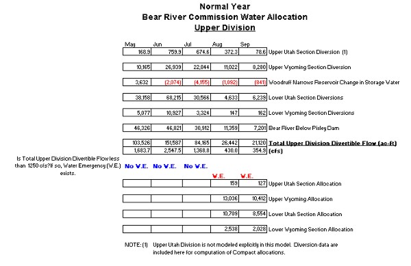
The "Bear River Commission Water Allocation: Central Division" table (Table 15) uses the Water Commissioner's worksheet to determine if a water emergency exists in the Central Division under the current scenario. If so, the worksheet computes the allocations for the State of Wyoming and Idaho are computed as defined in the Bear River Compact.
Table 15. Bear River Commission Water Allocation Worksheet: Central Division (Normal Hydrologic Conditions)
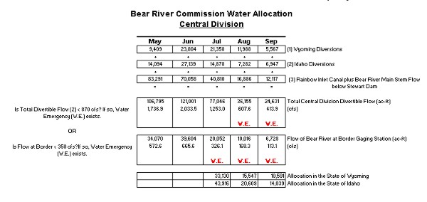
A spreadsheet model of the Bear River Basin was developed which simulates the operation and flows in the Bear River system. All significant diversions were modeled in addition to two tributaries, Sulphur Creek and Smiths Fork. Prior to use, a full analysis and calibration of the model is required to insure that the results of model scenarios properly reflect the hydrology and operational aspects of the basin. The calibration effort is contained in the Task 3C Memorandum, Surface Water Model Calibration.
The value of this model to users in the basin is in assessing the impact of proposed projects to the flows in the river. By simulating the river operations with and without the project, the change in flows can be analyzed for project benefits and system costs. This will be discussed in detail in the Task 3D Memorandum, Available Surface Water Determination.