Snake/Salt River Basin Water Plan
Final Report
TABLE OF CONTENTS
- III. AVAILABLE SURFACE WATER AND GROUNDWATER DETERMINATION
A. Surface Water Data Collection
B. Surface Water Model
C. Surface Water Availability
D. Ground Water Determination
E. Water Conservation
LIST OF FIGURES
Figure III-1. Annual Flows for USGS 13023000-Greys River above Reservoir near Alpine, Wyoming
Figure III-2. Annual Flows for USGS 13011900-Buffalo Fork above Lava Creek near Moran, Wyoming
Figure III-3. Snake River Node Diagram
Figure III-4. Salt River Node Diagram
Figure III-5. General Geology and Well Density
Figure III-6. Shallow Aquifer Recharge Rates
Figure III-7. USGS Ground Water Elevation Monitoring Sites
Figure III-8. Ground Water Permits for Domestic Use by Decade
Figure III-9. Wyoming State Engineer’s Office Permit Locations
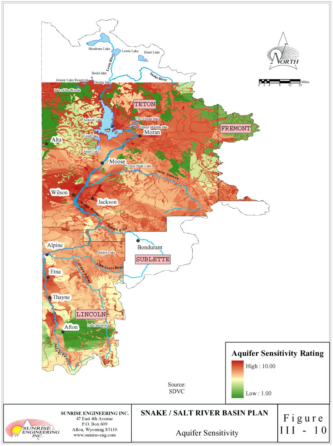
Figure III-10. Aquifer Sensitivity
III. AVAILABLE SURFACE WATER AND GROUNDWATER DETERMINATION
A. SURFACE WATER DATA COLLECTION
Introduction:
Prior to beginning the latest basin planning effort for the State, the Wyoming Water Development Commission (WWDC) considered the methods to be used for basin surface water modeling. They determined that three 12-month spreadsheet models (one each representing average-year, dry-year, and wet-year streamflows) constitute an appropriate level of detail for a modeling tool to verify existing uses and evaluate future surface water uses. Gage flows used in the three spreadsheets are to be typical of three different conditions, and are to be developed by averaging observed or estimated streamflows that occurred during historical average, wet, or dry years. Accordingly, the objectives of this task were to:
- collect historical records of streamflow from available sources
- determine the study period to be used to develop average, wet, and dry year flow
estimates for the Snake and Salt River basin spreadsheet models
- select indicator gages and use them to identify the historical average, wet, and
dry years out of the study period
- assemble surface water information required for the spreadsheet
Study Period Selection:
It is important in any water availability evaluation to select a study period that is long enough to include a variety of hydrologic conditions, including an extended period of dry years as well as wet years and average years. At the same time, it is important to avoid selecting a study period so long that many streamflows must be synthesized to fill-in missing data. Additionally, a single annual cycle will be used to model each hydrologic condition; therefore, the average data developed for input to the model should be derived from an operationally consistent time period. Construction of reservoir storage, changes in irrigation practices or change in water use (agricultural to suburban ranchette) are all significant in the study period selection.
Salt River
It is desirable in evaluating long-term hydrologic conditions to utilize streamflow records that have a long period of continuous record and reflect natural (virgin) flow, unaffected by upstream depletions or storage regulation. Unfortunately, no such streamflow gaging station exists in the Salt River basin. However, the Greys River above Reservoir, near Alpine gage has less than 500 acres of irrigated lands upstream of this gage (per USGS Water Resources Data) and has been in continuous operation since the 1954 water year. Since the irrigated acreage is small relative to the overall drainage basin (less than one percent), diversions were assumed to be small compared to the total natural flow. Therefore this gage was considered a natural flow gage and was used for the study period selection for the Salt River. The long term hydrograph is shown in Figure III-1.
Numerous irrigation systems were converted from flood to sprinkler systems during the late 1960's - early 1970's. Improvements in irrigation efficiencies ultimately impacted the overall watershed. Venn (2002) presented a double mass balance analysis of Salt River flows versus Greys River flows, showing a break in the trend line beginning in approximately 1971. He attributed the shift to changes in irrigation practice, from flood to sprinkler. This would suggest that the study period for the Salt River should begin no sooner than 1971. On the other hand, as no other major water developments have occurred in the Salt River basin since 1971, there's no reason to begin the study period any later in time.

Based on an evaluation of the long-term hydrologic conditions on the Greys River, together with an understanding of the availability of historical stream flow records and irrigation practices within the Salt River basin, a 31-year study period of 1971 through 2001 was selected as the candidate study period.
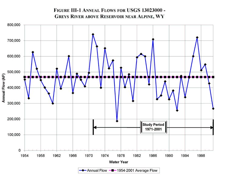
This selection was further supported by an analysis of the characteristics of the long term (1954-2001) record and the proposed study period (1971-2001). This information is tabulated below:
Table III-1
Characteristics of Annual Flow Series for
USGS 13023000 - Greys River above Reservoir, near Alpine, WY
|
1954-2001 |
1971-2001 |
| Mean (AF) |
468,627 |
478,985 |
| Standard Deviation |
128,603 |
143,253 |
| Three highest years |
1971 |
1997 |
1986 |
1971 |
1997 |
1986 |
| Three highest values (AF) |
740,050 |
720,160 |
708,630 |
740,050 |
720,160 |
708,630 |
| Three lowest years |
1977 |
1992 |
2001 |
1977 |
1992 |
2001 |
| Three lowest values (AF) |
187,390 |
255,120 |
267,035 |
187,390 |
255,120 |
267,035 |
Table III-1 shows that means of the two periods are very similar. Standard deviation for the shorter period is higher, which is to be expected for a smaller sample size. Most notably, the shorter study period includes both the three highest annual flows of record, as well as the three lowest.
Snake River
The Snake River near Moran gage has the longest period of record (1904-2001) of all the gages within the Snake River basin. However, this gage is located immediately downstream of Jackson Lake Dam, and measured flows are directly influenced by reservoir releases which makes it unsuitable for evaluating long-term hydrologic conditions within the Snake River basin. The Cache Creek near Jackson gage has no diversions upstream of the station and has been in continuous operation since 1963. However, it has a small drainage area (approximately 10.6 square miles) and as such, may not be representative of the overall basin. The Buffalo Fork above Lava Creek, near Moran gage has approximately 410 acres of land irrigated upstream of the gage and has been in operation since 1966. Because the irrigated acreage is small relative to the gage's drainage basin (less than one percent), this gage can be considered a natural flow gage. The long term hydrograph of the Buffalo Fork gage is presented in Figure III-2. There is no distinct time frame in which reservoir operations, irrigation, or other water use practices changed significantly within the Snake River basin. Jackson Lake was constructed at the mouth of a natural lake during 1910-11, and enlarged in 1916. The dam was modified in 1991 to correct dam safety deficiencies. This appears to have been accomplished without significantly impacting the reservoir's operations. Therefore, it would have been possible to use a longer study period in the Snake River basin than in the Salt, but in the interest of consistency, 1971-2001 was used for the Snake River as well.
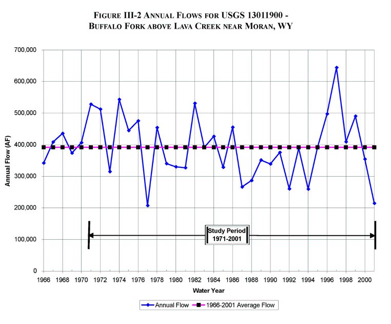
This selection is further supported by an analysis of the characteristics of the long term (1966-2001) record and the proposed study period (1971-2001). This information is tabulated below:
Table III-2
Characteristics of Annual Flow Series for
USGS 13011900 - Buffalo Fork above Lava Creek near Moran, WY
|
1966-2001 |
1971-2001 |
| Mean (AF) |
391,912 |
391,678 |
| Standard Deviation |
98,314 |
105,363 |
| Three highest years |
1997 |
1974 |
1982 |
1997 |
1974 |
1982 |
| Three highest values (AF) |
644,360 |
543,410 |
531,160 |
644,360 |
543,410 |
531,160 |
| Three lowest years |
1977 |
2001 |
1994 |
1977 |
2001 |
1994 |
| Three lowest values (AF) |
207,270 |
214,628 |
259,370 |
207,270 |
214,628 |
259,370 |
Table III-2 shows that means of the two periods are very similar. Standard deviation forthe shorter period is higher, which is to be expected for a smaller sample size. Most notably, the shorter study period includes both the three highest annual flows of record, as well as the three driest.
Indicator Gage Selection:
Approach
The periods of record for gaging stations in the basin were reviewed. Gages that operated throughout the study period were selected for evaluation as indicator gages. These gages were to provide annual flow characterization (average, wet, or dry) that could be applied to portions of the basin where long-term information did not exist. Table III-3 lists the gages that met this initial screening criterion.
Table III-3
Potential Indicator Gages for the Snake and Salt River Basins
USGS
Number |
Station Name |
Drainage
Area (mi2) |
Period of Record |
| From |
To |
| 13011000 |
Snake River near Moran, WY |
807.0 |
Sep-1903 |
Sep-2001 |
| 13011900 |
Buffalo Fork above Lava Creek near Moran, WY |
323.0 |
Sep-1965 |
Sep-2001 |
| 13018300 |
Cache Creek near Jackson, WY |
10.6 |
Jul-1962 |
Sep-2001 |
| 13022500 |
Snake River above Reservoir near Alpine, WY |
3465.0 |
Jul-1953 |
Sep-2001 |
| 13023000 |
Greys River above Reservoir near Alpine, WY |
448.0 |
Oct-1953 |
Sep-2001 |
| 13027500 |
Salt River above Reservoir, near Etna, WY |
829.0 |
Oct-1953 |
Sep-2001 |
The wettest and driest 20 percent of the study period years, on an annual basis, were identified for the gages listed above and are shown in Table III-4. To the extent possible, virgin flow gages, free from transbasin diversion, irrigation depletions, or storage regulation were desirable. Each potential indicator gage is discussed below:
Snake River near Moran, WY - As stated above, gages that are impacted by reservoir operations are not typically selected as an indicator gage. Located immediately below Jackson Lake, this gage reflects reservoir operations and would have required adjustment for change in reservoir storage and reservoir evaporation.
Buffalo Fork above Lava Creek near Moran, WY - This gage is one of the few long term gages that is minimally impacted by man's activities. Located very near the Snake River Moran gage, this gage was expected to reflect the same hydrologic conditions as the Snake River gage, without requiring adjustment. Therefore, average, wet, and dry year determinations from this gage record were applied to gages and headwater inflow nodes for the entire Snake River basin.
Cache Creek near Jackson, WY - Although this gage is also unaffected by man's activities, it was eliminated as an indicator gage because its small drainage area may not be hydrologically representative of larger sub-basins. For example, all other potential index gages have 1987 as a dry year. All except the Greys River have 1988 as a dry year as well. Cache Creek shows neither year as being dry. This gage was not selected as an indicator gage.
Snake River above Reservoir near Alpine, WY - This gage is significantly impacted by man's activities. It reflects reservoir deliveries from Jackson Lake to Palisades Reservoir, as well as all consumptive uses in the Snake River basin. Since it is not a virgin flow gage, it was not selected as an indicator gage.
Greys River above Reservoir, near Alpine, WY - This gage is minimally impacted by man's activities and can be assumed to be a virgin flow gage. Therefore, it was selected as an indicator gage. Average, wet and dry years determined from this gage were used to determine average, wet and dry year flows for the Salt River.
Salt River above Reservoir near Etna, WY - This gage is significantly impacted by man's activities. Since it is not a virgin flow gage, it was not selected as an indicator gage. The Greys River gage will serve as the indicator gage for the Salt River.
Results
In summary, the same two gages that served in determining study period of record became designated indicator gages for the study: Buffalo Fork above Lava Creek near Moran, WY, and Greys River above Reservoir, near Alpine, WY. If there had been additional suitable gages, more indicator gages could have been selected and applied to different sub-areas of the basin, but this was not the case.
Table III-4
Potential Indicator Gages for the Snake and Salt River Basins
|
|
71 |
72 |
73 |
74 |
75 |
76 |
77 |
78 |
79 |
80 |
81 |
82 |
83 |
84 |
85 |
86 |
87 |
88 |
89 |
90 |
91 |
92 |
93 |
94 |
95 |
96 |
97 |
98 |
99 |
00 |
01 |
| 13011000 |
Snake River near Moran, WY |
W |
N |
N |
W |
N |
N |
D |
D |
N |
N |
N |
N |
N |
W |
N |
W |
D |
D |
D |
D |
N |
N |
D |
N |
N |
W |
W |
N |
N |
N |
N |
| 13011900 |
Buffalo Fork above Lava Creek nearMoran,WY |
W |
W |
D |
W |
N |
N |
D |
N |
N |
N |
N |
W |
N |
N |
N |
N |
D |
D |
N |
N |
N |
D |
N |
D |
N |
W |
W |
N |
N |
N |
D |
| 13018300 |
Cache Creek near Jackson,WY |
W |
W |
N |
N |
N |
N |
D |
N |
N |
N |
N |
N |
N |
N |
D |
W |
N |
N |
N |
D |
D |
D |
N |
D |
N |
W |
W |
W |
N |
N |
D |
| 13022500 |
Snake River above Reservoir near Alpine, WY |
W |
W |
N |
W |
N |
N |
D |
N |
N |
N |
D |
N |
N |
N |
N |
W |
D |
D |
N |
N |
N |
D |
N |
D |
N |
W |
W |
N |
N |
N |
D |
| 13023000 |
Greys River above Reservoir near Alpine, WY |
W |
W |
N |
W |
N |
N |
D |
N |
N |
N |
D |
N |
W |
N |
N |
W |
D |
N |
N |
D |
N |
D |
N |
D |
N |
N |
W |
N |
N |
N |
D |
| 13027500 |
Salt River above Reservoir near Etna, WY |
W |
W |
N |
N |
N |
N |
D |
N |
N |
N |
D |
N |
W |
W |
N |
W |
D |
D |
N |
D |
N |
D |
N |
N |
N |
N |
W |
N |
N |
N |
D |
LEGEND
| Dry Year |
D |
| Wet Year |
W |
| Normal |
N |
Gage Filling and Data Extension:
Six gages in the Snake/Salt River basin, including the Greys River gage selected as an indicator gage, have complete records over the study period. The remaining gages required data filling or extension for all or part of the study period.
The mixed-station method described by Alley and Burns (1981) was used to fill the gage records for the Snake/Salt River Basin Models. Ayres Associates developed a Graphical User Interface for the Colorado Decision Support System as a front end to the USGS Mixed Station Model (Colorado River Decision Support System, 2000). This GUI and model were used to perform the data filling and extension.
The mixed station method allows the use of different independent gages to estimate gage flows for different missing members of a monthly time series. The Simple Linear Regression calculation option was used in this study. Accordingly, a simple linear regression model is developed for each independent gage with which a dependent gage has a common period of record. The regression that produces the smallest standard error of prediction (SEP) for a given month is then used to fill the missing data. The mixed station model also allows for either a cyclic or non-cyclic regression. The non-cyclic regression is developed from pairs of data for all months in the common record, and can be applied to any month. The cyclic approach, on the other hand, uses only same-month data pairs to develop a regression model for a given month. A minimum of five concurrent values was the threshold for use of the cyclic option. The smallest standard error is again the criterion to determine whether the cyclic or non-cyclic value is used. To fill gages in the Snake River basin, the set of independent gages was limited to those within the basin and the gage on the Greys River above the Reservoir at Alpine. Due to the fewer potential independent gages in the Salt River basin, all Snake and Salt basin gages were available in the filling of the Salt River basin gages.
Ungaged Tributary Inflow Estimation:
Several tributaries to the Snake and Salt Rivers, while included in the model network, do not have maintained gaging stations/records. It was therefore necessary to estimate average, wet, and dry year flows for these catchments as inflows to the models. Inflow was estimated for tributaries with sizable diversion rights. Flow contributions from tributaries that do not have modeled diversions were included in the basin gain calculation.
An average annual runoff for these catchments was estimated using regression equations derived for mountainous regions of Wyoming published in USGS WRIR 88-4045 (Lowham, 1988). Derived from several long-term gage records, these regression equations estimate annual average runoff from physical parameters of catchment area and average elevation, or area and average annual precipitation. For this study, the average basin elevation method was used because it is the more basin-specific method. Catchment areas and mean basin elevations were derived from USGS 1:100000 scale topographic maps. The average elevation regression equation is:
Qa=0.0015A^1.01(Elev/1000)^2.88
where,
Qa = annual runoff (cfs)
A = contributing area (mi2)
Elev = average basin elevation (feet)
Once average annual discharge values were calculated, it was necessary to derive monthly runoff values for the entire model period. This was done by correlation to a nearby gaging station with similar catchment characteristics. The derived monthly values are the product of the respective gaged monthly flow multiplied by the ratio of the annual ungaged and gaged discharges. Once the time series of estimated flows was created, average, wet, and dry years flows were calculated based on the respective indicator gage. Table III-5 presents the average annual runoff estimate using the above regression and the corresponding gage used in the distribution of flows for the Salt and Snake River basins.
In some cases the annual flow estimations appeared low in comparison to nearby gaged catchments. In the event that this resulted in shortages to diversions in the spreadsheet models, a second estimation method was used. In this case, a simple area weighting of the monthly flows of a similar watershed in close proximity was used. This was the case in Cedar Creek, Lee Creek, Birch Creek, and Stewart Creek in the Salt River basin. These tributary flows were estimated based on gaged flow in Strawberry Creek.
Summary and Conclusions:
- The model study period for both the Snake and Salt River basins is 1971-2001.
- The following indicator gage and applicable hydrological areas have been
selected:
- Buffalo Fork above Lava Creek near Moran, WY - Snake River basin
- Greys River above Reservoir near Alpine, WY - Salt River basin
- Gage records were filled using simple linear regression models selected by the
USGS Mixed Station Model.
- Ungaged headwater flows were developed using elevation-based regression
models; in a few cases this approach appeared inadequate and instead, nearby
gage flow was scaled by drainage area.
Table III-5 Ungaged Tributary Streamflow Estimates,
Methods of WRIR 88-4045
| Basin |
Catchment and Downstream Extent |
Drainage Area
(sq. mi.) |
Mean Basin
Elevation
(ft amsl) |
Estimated Annual Runoff
(Mean Basin Elevation
Method) |
1971-2001 Average Annual
Flow at Nearest Recording
Gage |
Notes |
Annual
Runoff AF |
Annual
Runoff
AF/sq.mi. |
Gage # |
Annual
Gaged
Runoff
AF/sq.mi. |
| Salt |
Spring Creek, S16 T31N R119W |
42.7 |
7532 |
16127 |
378 |
13025500 |
430 |
MBE Method used. |
| Stewart Creek, S22 T36N R119W1 |
7.9 |
7201 |
2595 |
330 |
13027000 |
2610 |
MBE Method was not used. Estimate based on Strawberry
Creek Flows. |
| Birch Creek, S36 T36N R119W |
2.8 |
8143 |
1270 |
460 |
13027000 |
2610 |
MBE Method was not used. Estimate based on Strawberry
Creek Flows. |
| Lee Creek, S12 T35N R119W2 |
6.66 |
8094 |
2976 |
452 |
13027000 |
2610 |
MBE Method was not used. Estimate based on Strawberry
Creek Flows. |
| Cedar Creek, S5 T34N R118W |
5.9 |
8216 |
2823 |
476 |
13027000 |
2610 |
MBE Method was not used. Estimate based on Strawberry
Creek Flows. |
| Willow Creek near Turnerville, S14 T33N R118W |
14.2 |
8333 |
7126 |
500 |
13027000 |
2610 |
MBE Method used. |
| Dry Creek, S8 T31N R118W |
20.5 |
8326 |
10250 |
501 |
13024500 |
1253 |
MBE Method used. |
| Toms Creek, S6 T32N R119W |
18.8 |
6651 |
4932 |
262 |
13025500 |
430 |
MBE Method used. |
| Stump Creek, S6 T32N R119W1 |
102.7 |
7226 |
34542 |
336 |
13025500 |
430 |
MBE Method used. |
| Snake |
Lava Creek, confluence with Buffalo Fork |
27.1 |
7995 |
12096 |
447 |
13011900 |
1213 |
MBE Method used. |
| Ditch Creek, confluence with Snake River |
63.2 |
7543 |
24078 |
381 |
13014500 |
634 |
MBE Method used. |
| Spring Creek, S13 T40N R117W |
13.1 |
6440 |
3121 |
238 |
13016450 |
1600 |
MBE Method used. |
| Fish Creek, S11 T41N R117W |
14.5 |
7680 |
5731 |
396 |
13016450 |
1600 |
MBE Method used. |
| Nowlin, Twin and Sheep Creeks, S11 T41N R116W |
32.9 |
7826 |
13846 |
421 |
13018000 |
848 |
MBE Method used. |
| Granite Creek (Hoback), confluence with Little Granite Creek |
61.5 |
8758 |
36003 |
586 |
13019500 |
925 |
MBE Method used. |
| Upper Hoback, confluence of Granite Creek |
367.9 |
7828 |
158831 |
432 |
13019438 |
1146 |
MBE Method used. |
Notes:
1. Calculations based on multiple sub-basins
2. Includes Green and Prater Canyons.
B. SURFACE WATER MODEL
The WWDC has undertaken water basin planning efforts throughout Wyoming. The purpose of the statewide planning process is to provide decision-makers with current, defensible data to allow them to manage water resources for the benefit of all the state's citizens. Spreadsheet models were developed to determine average monthly streamflow in the basin during normal, wet, and dry years. The purpose of these models was to validate existing basin uses, assist in determining the timing and location of water available for future development, and help to assess impacts of future water supply alternatives.
The WWDC specified that the models developed for the various Wyoming river basins be consistent, and use software available to the average citizen. Accordingly, Excel was selected as the platform to support the spreadsheet modeling effort. The spreadsheet model developed for the Bear River, the first basin plan undertaken, became a template for subsequent river basin modeling, and new features were added as unique circumstances were encountered in those basins. In this task, the spreadsheet models used in the Powder/Tongue River Basin Plan were used as a basis and were re-populated with Salt and Snake River node networks and associated data. The existing logic was adequate to express operations in these two basins, and there were no substantial changes to the spreadsheet logic.
This study encompassed creating and calibrating six spreadsheet workbooks, one for each of three hydrologic conditions and two distinct sub-basins:
- • Snake River from the headwaters near Jackson Lake to just above Palisades Reservoir
near Alpine, WY
- • Salt River from the headwaters to just above Palisades Reservoir near Alpine, WY
The three workbooks for each sub-basin are yoked together with a simple menu-driven graphical user interface (GUI), effectively creating two sub-basin models.
Model Overview:
For each Snake/Salt River sub-basin, three models were developed, reflecting each of three hydrologic conditions: dry, normal, and wet year water supply. The spreadsheets each represent one calendar year of flows, on a monthly time step. The modelers relied on historical gage data from 1971 to 2001 to identify the hydrologic conditions for each year in the study period. Because historical diversion data were virtually unavailable for this period, total diversions and resulting return flows were not explicitly included in the spreadsheets. Instead, only the consumptive portion of diversions is taken out of the stream in the models. Thus, streamflow and consumptive use are the basic input data to the model. For these data, average values drawn from the dry, normal, or wet subset of the study period were computed for use in the spreadsheets. The models do not explicitly account for water rights, appropriations, or compact allocations nor is the model operated based on these legal constraints. It is assumed that the limitations that may be placed on users due to water rights restrictions are reflected in the number of irrigating days included in the consumptive use calculations for each of the three hydrologic conditions.
To mathematically represent each sub-basin system, the river system was divided into reaches based primarily upon the location of major tributary confluences. Each reach was then sub-divided by identifying a series of individual nodes representing diversions, tributary confluences, gages, or other significant water resources features. The resulting network is the simplification of the real world that the model represents. Figure III-3 and Figure III-4 present node diagrams of the models developed for the Snake and Salt River sub-basins. The numbered nodes in the diagram represent primarily gage or inflow nodes and confluence nodes; the diagram does not depict diversion nodes.
Virgin flow for each month is supplied to the model by specifying flow at every headwater node, and incremental stream gains and losses within each downstream reach. Where available, upper basin gages were selected as headwater nodes; in their absence, flow at the ungaged headwater point was estimated outside the spreadsheet. For each reach, incremental stream gains (e.g., ungaged tributaries, groundwater inflow, and inflow resulting from human-caused but unmodeled processes) and losses (e.g. seepage, evaporation, and unspecified diversions) are computed by the spreadsheet. These are calculated by adding net modeled effects (diversions) within the reach back into the difference between the upstream and downstream historical gage flows. Stream gains are input at a point in the reach below the gaged or estimated inflow to be available for diversion downstream and losses are subtracted at the bottom of each reach.
At each node, a water budget computation is completed to determine the amount of water that flows downstream out of the node. The amount of flow available to the next node downstream is the difference between inflow, including upstream inflows, return flows, imports and reach gains, and outflows, including diversions, reach losses and exports. For the Snake/Salt Rivers, imports/exports and return flows are not modeled explicitly, but are set to zero in the water budget calculation. Diverted amounts at diversion nodes are the minimum of demand (consumptive use requirements) and physically available streamflow. Mass balance, or water budget, calculations are repeated for all nodes in a reach.
Model output includes the diversion demand and simulated diversions at each of the diversion points, and streamflow at each of the Snake/Salt River basin nodes. Impacts associated with various water projects can be estimated by changing input data, as decreases in available streamflow or as changes to diversions occur. New storage projects that alter the timing of streamflows or shortages may also be evaluated.
Model Structure and Components:
Each of the Snake/Salt River sub-basin models is a workbook consisting of numerous individual pages (worksheets). Each worksheet is a component of the model and completes a specific task required for execution of the model. There are five basic types of worksheets:
- Navigation Worksheets: Graphical User Interfaces (GUIs) containing buttons used to
move within the workbook;
- Input Worksheets: raw data entry worksheets (USGS Gage data or headwater inflow
data, Diversion Data, etc.);
- Computation Worksheets: compute various components of the model (gains/losses);
- Reach/Node Worksheets: calculate the water budget node by node; and
- Results Worksheets: tabulate and present the model output.
The delineation of a river basin by reaches and nodes is more an art than a science. The choice of nodes must consider the objectives of the study and the available data. It also must contain all the water resources features that govern the operation of the basin. The analysis of results and their adequacy in addressing the objectives of the study are based on the input data and the configuration of the river basin by the computer model.
The following reaches and nodes are contained in each basin model:
- Snake River basin: 30 reaches, 68 nodes
- Salt River basin: 27 reaches, 49 nodes
Gage Data:
Monthly stream gage data were obtained from the Wyoming Water Resources Data System (WRDS) and the USGS for each of the stream gages used in the model. Linear regression techniques were used to estimate missing values for the many gages that had incomplete records. The Mixed Station Model developed by the USGS was used to perform the regression and data filling. Once the gages were filled in for the study period, monthly values for dry, normal, and wet conditions were averaged from the dry, normal, or wet years of the study period. The dry, normal, and wet years were determined on a sub-basin level from indicator gages in each sub-basin.
Headwater inflow at several ungaged locations is also on the Gage Data worksheet. The model uses estimated flow at ungaged headwater nodes as if they were gages. Several approaches to estimating the flow were used, depending on the complexity of the stream system, availability of data, and reasonableness of fit. For instances where the contributing area above a stream gage was small, diversions above this gage were simply added to the gage to estimate the inflow to the reach. Regression equations for estimating streamflow in Wyoming (Lowham, 1988) were used in estimating the majority of the ungaged basins. However, there where occurrences when this appeared to underestimate streamflow, as indicated by an inability to meet reach diversions. In these cases, a third approach was used where a simple correlation to a nearby gaged basin was made.
Diversion Data:
Surface water diversions in the Snake/Salt River Basin Models are primarily for agricultural use, as municipal use is supplied from groundwater. Because actual diversion records were unavailable in these basins, the model simulates the depletion, that is, the consumptive portion of the diversion, being taken from the stream. Since the model treats this quantity as if it was the diverted amount, and for consistency with other basin spreadsheets, we refer to this information as "diversion data", although it is a depletion quantity.
Data on the diversion data sheet are used to calculate ungaged reach gains and losses, and in some cases, inflow at ungaged headwater nodes. They are also used as the diversion demand in the Reach/Node worksheets.
When diversions are modeled as depletions, overall mass balance of the system is preserved because the inefficient fraction of the diversion is accounted for in the calculated gain/loss term for the reach. For example, consider a ditch located in a reach that gains 1,000 AF one month from the upstream gage to the downstream gage, due to small tributary inflow, groundwater interaction, and other non-point contributions. The ditch diverts 100 AF during the month, consumes 33 AF, returns 40 AF to the stream this month, and returns 27 AF to the stream over the following months. Net depletion to the stream this month is 60 AF, meaning that 940 AF of the reach gain actually shows up at the downstream gage. From the model's perspective, the ditch diverts 33 AF, the reach gain is only 973 AF, and 940 AF of the reach gain shows up at the modeled downstream gage also.
Reach Gain/Loss:
The Snake/Salt River Basin Models simulate major diversions and features of the basins, but minor water features (e.g., small tributaries lacking historical records, diversions for small permitted acreage) are not explicitly included. Some features are aggregated and modeled, while the effects of many others are lumped together using a modeling construct called "ungaged reach gains and losses". These ungaged gains and losses account for all water in the budget that is not explicitly named and can reflect ungaged tributaries, groundwater/surface water interactions, lagged return flows associated with structures that divert consumptive use only in the model, or any other process not explicitly or perfectly modeled.
C. SURFACE WATER AVAILABLITY
Available supply per the spreadsheet model is further subject to compact limitations. The limitation is on basinwide annual use, based on total annual flow at the Idaho state line. As a practical matter, Wyoming's current post-compact diversions of approximately twenty thousand acre-feet can increase by five to ten times before the compact becomes limiting. However, in some parts of the basin, particularly on the Snake River main stem, the compact is much more limiting than the amount of water unappropriated within Wyoming. Furthermore, availability across the entire basin, once the compact is considered, is much less than the combined available supplies of the Snake and Salt Rivers, as defined by the spreadsheet analysis.
Available Flow (Spreadsheet Model Analysis):
Each basin model is divided into a number of reaches, each composed of several nodes, or water balance points. Reaches are typically defined by gages or confluences, and represent tributary basins or subsections of the main stem. An output worksheet in each spreadsheet model summarizes monthly flow at the downstream end of each reach, and provides the basis of this analysis. In general, simulated flow at the reach terminus indicates how much water is physically present, but it may not fully reflect flow that is available for future appropriation. This apparently "available flow" may already be appropriated to a downstream user, may be satisfying an instream flow right, or may result from reservoir storage water being delivered to specific points of diversion downstream. In short, it is important to acknowledge these existing demands when determining available flow.
To determine how much of the physical supply is actually available to future uses, physical supply at several reaches was first adjusted for the following circumstances:
- assumed approval of two pending instream flow right applications on Fish Creek, a tributary of the Snake River. The reaches covered by these permits fall within Reach 18 of the Snake River model, and call for 150 cfs of flow;
- assumed approval of a pending instream flow right application on the Salt River, in model reach 27, for 221 cfs;
- deliveries of storage water from Jackson Lake to Palisades Reservoir throughout the Snake River mainstem. Differentiating natural flow water from storage water requires a basic understanding of Jackson Lake and Minidoka Project operations, as well as some assumptions about operating conditions during Normal, Dry, and Wet years. The following subsection addresses these topics.
The "available flow" at each point is defined as the minimum of the physical supply value, adjusted to take into account the above-listed instream demands, and "available water" at all downstream reaches. In other words, if adjusted physical supply at the node is the limiting value, then all that water can be removed from the stream without impacting either instream demand at this location, or downstream appropriators. Thus water available for future appropriation must be defined first at the most downstream point, with upstream availability calculated in stream order. These calculations were made on a monthly basis, and annual availability was computed as the sum of monthly available water. Note that calculating annual availability in this way can yield a different value than applying the same logic to annual flows for each reach. The summation of monthly values is more accurate, reflecting constraints of downstream use on a monthly basis.
Jackson Lake Operations:
Jackson Lake is the most upstream main stem feature of the U.S. Bureau of Reclamation's (USBR's) Minidoka Project, which serves irrigators generally located along the Snake River from the Wyoming border to south central Idaho near Twin Falls. The project operates under flexible administration which allows water in storage to be credited to whichever water right has access to it, regardless of where the water is stored. For instance, water generated above Palisades Reservoir can be stored there under the more senior downstream American Falls Reservoir right at the beginning of the runoff season. If and when American Falls successfully fills physically, the water in Palisades reverts to Palisades' right and ownership. The objective is to keep water as high in the basin as possible, thereby maximizing the ability to distribute the supply and minimizing the risk of spilling water from lower reservoirs when upper reservoirs are unable to fill.
As another example, Jackson Lake under normal operations matches winter outflow to inflow in order to maintain flood control capacity in the reservoir as well as minimum fish flows in the river below the dam. When water is released while Jackson Lake water rights are in priority the “bypass” may be stored to Jackson Lake’s credit in a downstream reservoir. Another frequent situation occurs when water is delivered from Jackson Lake accounts but physically delivered from a downstream reservoir. Then, water released from Jackson Lake through the subsequent winter may already belong downstream.
Jackson Lake's operational year begins October 1st. Ideally the lake level is drawn down to 6760.95 feet, an elevation that provides 200,000 af of winter flood control space. Under these circumstances, outflows are set to match inflows, which in an average year might be on the order of 400 or 500 cfs. Wyoming has the option, to utilize its storage water supply from Palisades Reservoir to augment the stream flow, provided there is a commensurate amount of water in Wyoming's pool in Palisades Reservoir. The exchange water is reallocated within Palisades Reservoir to Jackson Lake spaceholders. When spring runoff begins, typically in April, storage begins gradually in accordance with flood control criteria covering both Jackson Lake and Palisades. These criteria take into consideration forecasted inflow, downstream flow limitations, and a specified division of the total required space between Jackson Lake and Palisades Reservoir. Target levels are re-computed daily as the hydrograph rises. The objectives are to maintain adequate space in the reservoirs to control runoff while flow is increasing, and complete filling during the receding limb of the hydrograph. Generally, filling is achieved by mid-June. For the remainder of the water year, the Bureau tries to maintain outflows as uniformly as possible to reach elevation 6760.95 by October 1st. In other words, over this period of a normal or wet year, they are moving inflows plus 200,000 AF down the river. In a dry year, they will move more storage water and Jackson Lake will be below 6760.95 feet on October 1st. In a normal or above normal year, releases rates are dictated by the need to evacuate for winter and spring flood control; in drier years, the rates may be more influenced by downstream demand.
To estimate the amount of water available to a new appropriator on the Snake River main stem, certain assumptions were made regarding normal, wet, and dry year operations. These assumptions are extremely general, since in any given year, circumstances are unique. In particular, antecedent conditions bear greatly on annual operations, as a wet year following a dry or normal year is operationally different from a wet year following a wet year. Furthermore, these generalizations are based on historical practice, which has neither required strict administration of the river nor forced resolution of potential conflicts in perspective between Wyoming and USBR. With that in mind, these scenarios were envisioned for each modeled hydrologic condition:
Normal Year
October -March: all flows immediately below Jackson Lake Dam are project deliveries, and cannot be appropriated.
April - June: filling at both Jackson Lake and Palisades Reservoir is in accordance with flood control operations; outflows from Jackson Lake are excesses that can't be stored, and any amount above the 280 cfs fishery requirement is available to appropriators.
July-September: 200,000/3=66,666 AF/mo of flow below Jackson Lake are project deliveries and cannot be appropriated; the balance is available to appropriators.
Wet Year
October-December: all flows immediately below Jackson Lake Dam are project deliveries, but…
January - March: …as winter progresses it becomes evident that spring flows will be high. Palisades Reservoir no longer stores water coming past Jackson Lake, and it may be appropriated.
April-June: outflows from Jackson Lake are excesses that can't be stored, and any amount above 280 cfs is available to appropriators.
July - September: 200,000/3=66,666 AF/mo of flow below Jackson Lake are project deliveries and cannot be appropriated; the balance is available to appropriators.
Dry Year
October-March: winter outflows from Jackson Lake are project flows, and cannot be appropriated.
April-May: flows immediately below Jackson Lake are excesses that can't be stored; runoff ends early and the reservoir may or may not have achieved fill.
June - September: approximately 477,000/4 = 120,000 AF/mo are project deliveries, and the balance can be appropriated. The value 477,000 AF is the sum of 200,000 AF out of the flood control/irrigation pool, and an additional 277,000 AF out of storage. The latter value is the average annual change in storage for four recent dry years (1973, 1977, 1992, 1994).
Results:
Tables III-7 through III-12 summarize available water for the two sub-basins and three hydrologic conditions. The shaded reaches are mainstem reaches. These tables take into account instream flow requirements and Jackson Lake operations as described above, as well as downstream appropriation. For instance, the proposed Salt River instream flow permit is in the most downstream model reach. Even though it has the greatest physical supply, the available supply is limited to flows above 221 cfs (approximately 13,000 AF/mo). Table III-10 shows that available supply is estimated as 20,904 AF in June of a dry year. The available supply at all upstream nodes is likewise limited to 20,904 AF in June; if more water was removed from the river in the upstream reach, the 221 cfs would be violated at the instream flow reach. The available water determination was estimated in a spreadsheet separate from the models themselves.
Table III-6 shows annual available supply at the most downstream node for each basin as follows:
TABLE III-6 ANNUAL AVAILABLE FLOW AT DOWNSTREAM NODE
| Dry Year
(AF/yr) | Normal Year
(AF/yr) | Wet Year
(AF/yr) |
| Snake River | 1,768,960 | 2,887,630 | 4,158,807 |
| Salt River | 216,249 | 458,153 | 694,494 |
These numbers represent much more water than can actually be developed, because of the Snake River Compact. The next section describes the compact and presents an estimate of the basinwide future development permitted under the compact.
Compact Limitations:
The compact protects all Wyoming rights that existed on July 1, 1949. It further permits Wyoming to divert, for new development post-1949, 4% of the Wyoming-Idaho state line flow of the Snake River. Domestic and stock uses are exempt from the limitation, and out-of-basin exports are not permitted without Idaho's permission. Wyoming can develop the first half of the 4% without providing anything additional to Idaho. To develop the second half, however, Wyoming must provide replacement storage space for Idaho's use to the extent of one-third of the second half of the diversions allowed by the Compact. This provision is expected to be addressed by Wyoming's 33,000 acre-foot pool in Palisades Reservoir, at whatever time Wyoming's post-compact use exceeds 2% of the state line flows. To date, this has not happened.
The Snake River Compact does not formally designate a commission as do some western interstate compacts. As a result, Wyoming and Idaho do not meet on a regular basis under the auspices of the compact. As shown later in the report in Table III-13, Wyoming has not yet reached the final 2% of its allocation.
For this study, an estimate was made of compact limitations on future development under the three hydrologic conditions. This approach is appropriate because the Compact does not refer to rolling average limitations that would permit average limits in years of less-than-average supply. The first step was to estimate the amount of post-compact use during the study period. This was done by assuming that the fraction of post-1949 adjudicated rights among all adjudicated rights also represents the amount of post-compact use among all use. The "post-compact fraction" was determined to be 4 percent in the Salt River basin, and 13 percent in the Snake River basin. Actual basis of the computation was adjudicated acres associated with each right. Post-compact depletions for each hydrologic condition were then calculated as the post-compact fraction multiplied by the depletion modeled in each spreadsheet model. Post-compact depletions on the Greys River were assumed to be negligible, as there has been no significant development in the basin over the last five decades.
State line flow was calculated next for each hydrologic condition, as specified in Article III of the compact. Specifically, the quantity of water crossing the State line was computed as the sum of annual flows for USGS gages Snake River above Reservoir near Alpine (13022500), Salt River above Reservoir near Etna (13027500), and Greys River above Reservoir, near Alpine (13023000). Annual change in storage in reservoirs that serve Idaho (i.e., Jackson Lake) was assumed to be zero in normal and wet years, and -277,000 acre-feet in dry years. This number is the average of the historical annual change for water years 1973, 1977, 1992, and 1994. (Values for 1987 and 1988 were not representative because of construction on Jackson Lake Dam.) The sum of the terms gage flow, change in storage, and post-compact depletions, is the amount of water to which 4% is applied in order to determine compact limits.
Once the compact limitation was computed, current post-compact diversions needed to be subtracted from the upper limit in order to estimate the remaining diversion allowance. A factor of 3.0 was used to convert depletions to diversions, based on logic implicit in the compact. The compact specifies that pre-compact flow be computed by adding one-third of the post-compact diversions to the state line gage flow; and that Wyoming's replacement duty to Idaho, once the first half of the compact allowance has been used, is one-third of post-compact diversions. These terms indicate that depletion to the river is generally accepted to be one-third of the diversion amount, with the remaining two-thirds of the diversion eventually returning to the stream.
Table III-13 summarizes the computations described above. It shows that the remaining allowable surface diversions from the basin are 90,000 AF/yr, 155,000 AF/yr, and 221,000 AF/yr in dry, normal, and wet years respectively.
Conclusion:
Surface water availability in the Snake and Salt River basins is a matter of physical supply, availability with respect to others' uses, and basinwide compact limits. In both the Salt and Snake basins, a new appropriation in a tributary basin will be limited by local supply, and without storage, may be severely limited in some months of the year. On the other hand, overall water supply in the basin greatly exceeds current use. On the main stems of both rivers, and in the larger tributaries of the Snake, the compact is more limiting than physical supply relative to existing demand. There are locations and months in which the entire annual compact allowance could be diverted within one month. Thus the supply available to any given proposed use varies greatly across the basin, and could be impacted by concurrent development of the compact allowance elsewhere in the basin.
Table III-7
Available Flow for Snake River Basin and Dry Hydrologic Condition
(values in acre-feet)
| Rch | Reach Name | Jan | Feb | Mar | Apr | May | Jun | Jul | Aug | Sep | Oct | Nov | Dec | Annual |
| 1 | Snake River near
Moran | 0 | 0 | 0 | 2,705 | 83,502 | 59,095 | 58,458 | 63,011 | 0 | 0 | 0 | 0 | 266,770 |
| 2 | Pacific Creek near Moran | 2,548 | 2,434 | 3,041 | 12,071 | 43,812 | 20,873 | 6,201 | 3,166 | 2,704 | 4,259 | 3,366 | 2,828 | 107,302 |
| 3 | Snake River below Pacific Creek | 3,812 | 3,650 | 3,870 | 16,302 | 131,888 | 81,305 | 67,387 | 67,708 | 4,553 | 5,998 | 4,851 | 4,040 | 395,364 |
| 4 | Buffalo Fork above Lava Creek | 7,409 | 6,494 | 7,353 | 15,560 | 55,594 | 77,825 | 25,091 | 12,691 | 9,617 | 13,226 | 10,041 | 8,268 | 249,169 |
| 5 | Lava Creek | 244 | 214 | 242 | 513 | 2,113 | 2,459 | 743 | 349 | 308 | 436 | 331 | 272 | 8,224 |
| 6 | Buffalo Fork below Lava Creek | 8,012 | 7,367 | 10,175 | 18,902 | 55,594 | 106,193 | 36,420 | 12,997 | 10,093 | 14,711 | 11,221 | 9,275 | 300,962 |
| 7 | Snake River below Buffalo Fork | 11,824 | 11,017 | 14,044 | 35,204 | 187,482 | 187,499 | 103,807 | 80,704 | 14,646 | 20,709 | 16,073 | 13,315 | 696,326 |
| 8 | Spread Creek | 1,057 | 927 | 1,049 | 2,220 | 8,891 | 9,752 | 2,497 | 917 | 1,255 | 1,887 | 1,433 | 1,180 | 33,066 |
| 9 | Snake River below Spread Creek | 17,800 | 16,678 | 18,319 | 43,365 | 214,177 | 202,456 | 116,923 | 87,579 | 23,098 | 29,364 | 23,284 | 19,214 | 812,259 |
| 10 | Ditch Creek | 748 | 641 | 666 | 988 | 4,613 | 2,419 | 607 | 222 | 560 | 985 | 735 | 731 | 13,915 |
| 11 | Snake River below Ditch Creek | 29,446 | 27,805 | 26,130 | 57,514 | 257,909 | 215,401 | 140,255 | 100,389 | 39,569 | 45,339 | 36,820 | 30,399 | 1,006,976 |
| 12 | Gros Ventre River | 10,695 | 9,421 | 11,063 | 15,309 | 65,475 | 40,122 | 13,807 | 9,138 | 8,973 | 15,787 | 11,883 | 11,386 | 223,059 |
| 13 | Snake River between Gros Ventre and Fish Creek | 40,141 | 37,226 | 37,193 | 72,823 | 310,940 | 254,774 | 153,466 | 109,072 | 48,518 | 61,126 | 48,703 | 41,785 | 1,215,767 |
| 14 | Lake Creek | 0 | 0 | 0 | 0 | 4,781 | 9,747 | 3,738 | 1,417 | 0 | 0 | 0 | 0 | 19,682 |
| 15 | Granite Creek | 0 | 0 | 0 | 0 | 4,781 | 5,187 | 1,648 | 389 | 0 | 0 | 0 | 0 | 12,004 |
| 16 | Lake Creek below Granite Creek | 0 | 0 | 0 | 0 | 4,781 | 14,255 | 5,177 | 1,646 | 0 | 0 | 0 | 0 | 25,858 |
| 17 | Fish Creek | 0 | 0 | 0 | 0 | 646 | 982 | 785 | 441 | 0 | 0 | 0 | 0 | 2,854 |
| 18 | Fish Creek below Lake Creek | 0 | 0 | 0 | 0 | 4,781 | 14,255 | 9,291 | 1,765 | 0 | 0 | 0 | 0 | 30,091 |
| 19 | Snake River below Fish Creek | 42,837 | 39,632 | 41,173 | 77,987 | 310,940 | 274,730 | 160,025 | 121,126 | 56,360 | 67,663 | 53,387 | 45,713 | 1,291,572 |
| 20 | Spring Creek | 193 | 248 | 691 | 663 | 170 | 0 | 0 | 372 | 348 | 861 | 672 | 514 | 4,732 |
| 21 | Snake River below Spring Creek | 44,751 | 42,505 | 50,253 | 86,167 | 310,940 | 274,730 | 160,025 | 127,904 | 58,936 | 78,364 | 61,899 | 52,090 | 1,348,564 |
| 22 | Flat Creek | 540 | 474 | 591 | 563 | 4,336 | 4,553 | 2,246 | 1,455 | 1,080 | 1,045 | 728 | 602 | 18,214 |
| 23 | Cache Creek | 446 | 383 | 431 | 646 | 1,341 | 1,093 | 735 | 475 | 402 | 675 | 593 | 532 | 7,751 |
| 24 | Flat Creek below Cache Creek | 3,242 |
3,166 | 3,360 | 3,997 | 5,036 | 4,553 | 4,125 | 2,724 |
2,755 | 4,054 | 3,793 |
3,472 | 44,278 |
| 25 | Snake River below Flat Creek | 47,993 | 45,671 | 53,612 | 90,165 | 310,940 | 274,730 | 160,025 | 130,520 | 61,685 | 82,418 | 65,692 | 55,562 | 1,379,013 |
| 26 | Hoback River | 11,297 | 9,417 | 8,974 | 26,048 | 87,413 | 50,540 | 20,244 | 13,510 | 10,847 | 14,621 | 11,757 | 10,412 | 275,080 |
| 27 | Little Granite Creek | 322 | 279 | 368 | 1,500 | 4,935 | 2,476 | 1,067 | 570 | 408 | 524 | 410 | 369 | 13,227 |
| 28 | Granite Creek | 2,125 | 1,781 | 1,792 | 5,603 | 18,868 | 10,956 | 4,651 | 3,010 | 2,147 | 2,849 | 2,280 | 2,026 | 58,089 |
| 29 | Hoback River below Granite Creek | 13,422 | 11,198 | 10,765 | 31,651 | 106,281 | 61,496 | 24,896 | 16,520 | 12,994 | 17,471 | 14,037 | 12,437 | 333,168 |
| 30 | Snake River below Hoback River | 63,907 | 59,831 | 70,339 | 133,269 | 408,526 | 342,169 | 192,112 | 151,226 | 79,449 | 107,730 | 86,484 | 73,917 | 1,768,960 |
Table III-8
Available Flow for Snake River Basin and Normal Hydrologic Condition
(values in acre-feet)
| Rch | Reach Name | Jan | Feb | Mar | Apr | May | Jun | Jul | Aug | Sep | Oct | Nov | Dec | Annual |
| 1 | Snake River near Moran | 0 | 0 | 0 | 42,162 | 131,888 | 204,061 | 84,674 | 78,272 | 55,388 | 0 | 0 | 0 | 596,444 |
| 2 | Pacific Creek near Moran | 2,686 | 2,673 | 3,487 | 10,715 | 61,683 | 74,049 | 19,878 | 5,942 | 4,204 | 3,839 | 3,255 | 3,010 | 195,422 |
| 3 | Snake River below Pacific Creek | 3,984 | 3,950 | 4,420 | 54,320 | 196,817 | 283,046 | 111,211 | 87,672 | 62,565 | 5,955 | 4,746 | 4,614 | 823,300 |
| 4 | Buffalo Fork above Lava Creek | 7,448 | 6,732 | 7,830 | 13,032 | 59,337 | 130,171 | 82,477 | 26,195 | 15,323 | 13,086 | 9,992 | 8,351 | 379,972 |
| 5 | Lava Creek | 245 | 222 | 258 | 429 | 1,937 | 4,207 | 2,873 | 801 | 500 | 431 | 329 | 275 | 12,508 |
| 6 | Buffalo Fork below Lava Creek | 8,130 | 7,539 | 11,538 | 18,635 | 85,144 | 170,867 | 82,477 | 27,059 | 16,459 | 13,359 | 10,832 | 9,362 | 461,400 |
| 7 | Snake River below Buffalo Fork | 12,115 | 11,489 | 15,958 | 72,956 | 281,961 | 453,913 | 193,688 | 114,731 | 79,024 | 19,313 |
15,578 | 13,976 | 1,284,700 |
| 8 | Spread Creek | 1,063 | 961 | 1,117 | 1,860 | 8,227 | 17,512 | 11,698 | 2,943 | 2,127 | 1,867 | 1,426 | 1,192 | 51,993 |
| 9 | Snake River below Spread Creek | 18,231 | 17,421 | 20,704 | 80,431 | 302,821 | 490,635 | 231,302 | 131,131 | 92,724 | 29,413 | 22,806 | 21,410 | 1,459,031 |
| 10 | Ditch Creek | 748 | 644 | 673 | 1,076 | 6,064 | 6,772 | 2,120 | 839 | 919 | 898 | 738 | 737 | 22,228 |
| 11 | Snake River below Ditch Creek | 30,174 | 29,080 | 29,417 | 93,947 | 336,558 | 539,158 | 289,989 | 161,210 | 119,255 | 48,549 | 36,397 | 35,975 | 1,749,710 |
| 12 | Gros Ventre River | 11,512 | 10,025 | 11,768 | 17,047 | 84,390 | 98,646 | 36,651 | 16,159 | 13,025 | 14,598 | 12,433 | 11,271 | 337,525 |
| 13 | Snake River between Gros Ventre and Fish Creek | 41,686 | 39,105 | 41,185 | 110,994 | 404,331 | 637,204 | 326,011 | 176,944 | 132,260 | 63,147 | 48,830 | 47,246 | 2,068,944 |
| 14 | Lake Creek | 0 | 0 | 0 | 0 | 3,163 | 15,080 | 10,177 | 2,374 | 0 | 0 | 0 | 0 | 30,794 |
| 15 | Granite Creek | 0 | 0 | 0 | 0 | 3,163 | 10,209 | 6,224 | 1,325 | 0 | 0 | 0 | 0 | 20,921 |
| 16 | Lake Creek below Granite Creek | 0 | 0 | 0 | 0 | 3,163 | 21,810 | 16,181 | 2,374 | 0 | 0 | 0 | 0 | 43,527 |
| 17 | Fish Creek | 0 | 0 | 0 | 0 | 566 | 1,400 | 1,211 | 479 | 0 | 0 | 0 | 0 | 3,656 |
| 18 | Fish Creek below Lake Creek | 0 | 0 | 0 | 0 | 3,163 | 21,810 | 17,903 | 2,374 | 0 | 0 | 0 | 0 | 45,249 |
| 19 | Snake River below Fish Creek | 45,175 | 42,162 | 45,895 | 118,362 | 404,331 | 659,592 | 354,498 | 188,852 | 141,081 | 69,232 | 53,991 | 51,077 | 2,174,247 |
| 20 | Spring Creek | 469 | 437 | 898 | 886 | 131 | 307 | 799 | 122 | 225 | 855 | 842 | 450 | 6,422 |
| 21 | Snake River below Spring Creek | 51,028 | 47,692 | 57,889 | 129,120 | 404,331 | 659,592 | 363,563 | 191,425 | 141,306 | 80,008 | 64,944 | 56,509 | 2,247,406 |
| 22 | Flat Creek | 597 | 538 | 570 | 771 | 3,830 | 7,686 | 6,545 | 3,302 | 1,786 | 945 | 725 | 675 | 27,971 |
| 23 | Cache Creek | 455 | 408 | 444 | 625 | 1,644 | 2,736 | 1,568 | 977 | 637 | 631 | 550 | 500 | 11,175 |
| 24 | Flat Creek below Cache Creek | 3,313 | 3,206 | 3,342 | 3,957 | 5,316 | 7,686 | 6,545 | 8,678 | 4,777 | 3,935 | 3,673 | 3,445 | 57,874 |
| 25 | Snake River below Flat Creek | 54,341 | 50,899 | 61,231 | 133,077 | 404,331 | 659,592 | 369,958 | 200,002 | 142,551 | 83,943 | 68,617 | 59,954 | 2,288,496 |
| 26 | Hoback River | 11,284 | 9,433 | 9,621 | 31,621 | 113,844 | 121,631 | 58,311 | 24,211 | 16,015 | 14,710 | 11,352 | 10,578 | 432,610 |
| 27 | Little Granite Creek | 336 | 312 | 431 | 1,828 | 7,557 | 7,478 | 2,579 | 1,027 | 602 | 533 | 441 | 387 | 23,512 |
| 28 | Granite Creek | 2,135 | 1,815 | 1,955 | 6,809 | 25,571 | 26,995 | 12,229 | 5,144 | 3,160 | 2,872 | 2,244 | 2,069 | 92,997 |
| 29 | Hoback River below Granite Creek | 13,419 | 11,248 | 11,576 | 38,429 | 139,415 | 148,626 | 70,540 | 29,354 | 19,175 | 17,582 | 13,597 | 12,647 | 525,607 |
| 30 | Snake River below Hoback River | 68,639 | 63,338 | 78,241 | 186,363 | 549,212 | 802,257 | 452,941 | 241,794 | 172,641 | 108,635 | 87,544 | 76,025 | 2,887,630 |
Table III-9
Available Flow for Snake River Basin and Wet Hydrologic Condition
(values in acre-feet)
| Rch | Reach Name | Jan | Feb | Mar | Apr | May | Jun | Jul | Aug | Sep | Oct | Nov | Dec | Annual |
| 1 | Snake River near Moran | 17,452 | 22,588 | 59,682 | 158,882 | 235,554 | 271,196 | 150,220 | 104,691 | 73,363 | 0 | 0 | 0 | 1,093,627 |
| 2 | Pacific Creek near Moran | 3,039 | 2,976 | 3,847 | 8,237 | 77,163 | 132,916 | 43,183 | 8,144 | 5,287 | 3,883 | 3,306 | 3,306 | 295,286 |
| 3 | Snake River below Pacific Creek | 21,970 | 26,982 | 64,520 | 168,208 | 315,597 | 414,148 | 194,529 | 117,677 | 81,921 | 6,113 | 4,987 | 4,789 | 1,421,442 |
| 4 | Buffalo Fork above Lava Creek | 7,644 | 6,450 | 8,163 | 12,079 | 68,471 | 209,157 | 129,563 | 39,252 | 20,895 | 13,137 | 10,781 | 9,064 | 534,657 |
| 5 | Lava Creek | 252 | 213 | 269 | 398 | 2,236 | 6,814 | 4,181 | 1,239 | 693 | 433 | 355 | 299 | 17,380 |
| 6 | Buffalo Fork below Lava Creek | 8,631 | 7,970 | 12,671 | 16,081 | 97,037 | 247,841 | 167,630 | 39,252 | 20,895 | 13,916 | 11,063 | 9,778 | 652,766 |
| 7 | Snake River below Buffalo Fork | 30,602 | 34,952 | 77,191 | 184,289 | 412,635 | 661,990 | 362,159 | 156,929 | 102,817 | 20,029 | 16,049 | 14,566 | 2,074,207 |
| 8 | Spread Creek | 1,091 | 920 | 1,165 | 1,724 | 9,505 | 28,840 | 17,350 | 4,794 | 2,966 | 1,875 | 1,539 | 1,293 | 73,063 |
| 9 | Snake River below Spread Creek | 37,453 | 41,393 | 82,214 | 190,250 | 433,350 | 729,891 | 383,896 | 180,568 | 118,516 | 30,582 | 24,130 | 21,631 | 2,273,872 |
| 10 | Ditch Creek | 757 | 654 | 684 | 1,146 | 8,298 | 10,295 | 4,152 | 1,202 | 1,136 | 909 | 748 | 738 | 30,718 |
| 11 | Snake River below Ditch Creek | 50,971 | 54,276 | 91,446 | 200,782 | 466,132 | 825,970 | 396,928 | 222,926 | 147,838 | 50,714 | 39,372 | 35,154 | 2,582,509 |
| 12 | Gros Ventre River | 12,507 | 10,519 | 12,589 | 19,456 | 115,267 | 147,528 | 69,706 | 21,015 | 15,992 | 14,911 | 13,236 | 12,807 | 465,532 |
| 13 | Snake River between Gros Ventre and Fish Creek | 63,478 | 64,795 | 104,035 | 220,238 | 581,141 | 972,942 | 466,012 | 243,502 | 163,814 | 65,625 | 52,608 | 47,961 | 3,046,150 |
| 14 | Lake Creek | 0 | 0 | 0 | 0 | 5,512 | 25,624 | 14,540 | 3,478 | 859 | 0 | 0 | 0 | 50,012 |
| 15 | Granite Creek | 0 | 0 | 0 | 0 | 4,639 | 16,238 | 9,019 | 1,849 | 859 | 0 | 0 | 0 | 32,603 |
| 16 | Lake Creek below Granite Creek | 0 | 0 | 0 | 0 | 5,512 | 25,624 | 21,655 | 4,742 | 859 | 0 | 0 | 0 | 58,392 |
| 17 | Fish Creek | 0 | 0 | 0 | 0 | 678 | 1,603 | 1,402 | 595 | 489 | 0 | 0 | 0 | 4,767 |
| 18 | Fish Creek below Lake Creek | 0 | 0 | 0 | 0 | 5,512 | 25,624 | 21,655 | 4,742 | 859 | 0 | 0 | 0 | 58,392 |
| 19 | Snake River below Fish Creek | 67,997 | 68,313 | 109,452 | 231,611 | 581,576 | 1,007,756 | 502,480 | 257,298 | 173,592 | 72,591 | 58,493 | 53,258 | 3,184,417 |
| 20 | Spring Creek | 764 | 561 | 1,126 | 1,445 | 173 | 635 | 2,534 | 0 | 254 | 929 | 1,066 | 959 | 10,447 |
| 21 | Snake River below Spring Creek | 77,989 | 75,578 | 124,677 | 249,403 | 581,576 | 1,010,854 | 535,061 | 257,298 | 173,847 | 84,168 | 72,618 | 65,964 | 3,309,034 |
| 22 | Flat Creek | 557 | 471 | 594 | 1,230 | 4,753 | 10,703 | 7,165 | 4,220 | 2,372 | 949 | 781 | 659 | 34,455 |
| 23 | Cache Creek | 508 | 446 | 476 | 595 | 2,188 | 4,791 | 2,050 | 1,282 | 811 | 669 | 577 | 546 | 14,940 |
| 24 | Flat Creek below Cache Creek | 3,236 | 3,095 | 3,289 | 4,063 | 5,960 | 10,703 | 7,165 | 11,375 | 5,004 | 3,726 | 3,542 | 3,384 | 64,543 |
| 25 | Snake River below Flat Creek | 81,225 | 78,674 | 127,966 | 253,465 | 581,576 | 1,021,425 | 542,079 | 259,346 | 176,207 | 87,894 | 76,160 | 69,349 | 3,355,366 |
| 26 | Hoback River | 11,415 | 9,541 | 10,132 | 35,372 | 158,232 | 181,502 | 78,499 | 31,976 | 18,600 | 15,082 | 11,461 | 11,046 | 572,859 |
| 27 | Little Granite Creek | 352 | 318 | 476 | 2,066 | 11,670 | 15,009 | 3,499 | 1,187 | 707 | 542 | 480 | 429 | 36,734 |
| 28 | Granite Creek | 2,171 | 1,838 | 2,079 | 7,635 | 36,582 | 43,639 | 16,342 | 6,556 | 3,673 | 2,941 | 2,298 | 2,183 | 127,937 |
| 29 | Hoback River below Granite Creek | 13,587 | 11,378 | 12,211 | 43,008 | 194,814 | 225,142 | 94,841 | 38,532 | 22,273 | 18,023 | 13,759 | 13,229 | 700,796 |
| 30 | Snake River below Hoback River | 96,597 | 91,073 | 146,069 | 304,925 | 787,383 | 1,254,196 | 656,220 | 314,777 | 216,648 | 110,129 | 94,621 | 86,169 | 4,158,807 |
Table III-10
Available Flow for Salt River Basin and Dry Hydrologic Condition
(values in acre-feet)
| Rch | Reach Name | Jan | Feb | Mar | Apr | May | Jun | Jul | Aug | Sep | Oct | Nov | Dec | Annual |
| 1 | Salt River near Smoot | 334 | 264 | 537 | 1,526 | 6,623 | 6,854 | 3,331 | 2,460 | 1,616 | 811 | 490 | 401 | 25,247 |
| 2 | Cottonwood Creek near Smoot | 1,043 | 842 | 836 | 1,628 | 3,415 | 2,408 | 1,193 | 1,417 | 1,331 | 1,312 | 1,151 | 1,088 | 17,664 |
| 3 | Salt River below Cottonwood Creek Confluence | 1,377 | 1,106 | 1,374 | 3,201 | 13,365 | 15,752 | 8,144 | 6,493 | 4,378 | 2,258 | 1,641 | 1,489 | 60,577 |
| 4 | Dry Creek near Afton | 324 | 262 | 260 | 502 | 962 | 0 | 0 | 203 | 380 | 408 | 358 | 338 | 3,997 |
| 5 | Salt River below Dry Creek Confluence | 1,701 | 1,368 | 1,634 | 3,734 | 16,514 | 19,876 | 10,413 | 8,376 | 5,700 | 2,756 | 1,999 | 1,828 | 75,897 |
| 6 | Swift Creek near Afton | 2,006 | 1,798 | 2,012 | 2,850 | 6,458 | 7,275 | 2,903 | 2,388 | 2,395 | 3,109 | 2,343 | 2,290 | 37,827 |
| 7 | Salt River below Swift Creek Confluence | 3,707 | 3,166 | 3,646 | 6,612 | 24,991 | 20,904 | 11,357 | 9,052 | 8,965 | 5,946 | 4,342 | 4,118 | 106,805 |
| 8 | Spring Creek (trib to Crow Creek) | 826 | 614 | 858 | 1,173 | 1,112 | 988 | 842 | 825 | 664 | 930 | 921 | 784 | 10,536 |
| 9 | Crow Creek near Fairview | 2,529 | 1,879 | 2,628 | 3,595 | 3,438 | 3,285 | 2,768 | 2,608 | 2,045 | 2,848 | 2,820 | 2,402 | 32,844 |
| 10 | Crow Creek below Spring Creek Confluence | 3,355 | 2,493 | 3,485 | 4,801 | 7,148 | 8,417 | 5,718 | 5,222 | 3,841 | 3,890 | 3,740 | 3,186 | 55,298 |
| 11 | Salt River below Crow Creek Confluence | 7,062 | 5,659 | 7,132 | 11,413 | 28,521 | 20,904 | 11,357 | 9,052 | 11,235 | 9,836 | 8,082 | 7,304 | 137,555 |
| 12 | Stump Creek | 1,769 | 1,314 | 1,837 | 2,508 | 2,248 | 1,078 | 1,054 | 1,449 | 1,377 | 1,992 | 1,972 | 1,680 | 20,278 |
| 13 | Salt River below Stump Creek | 8,152 | 6,794 | 7,975 | 13,942 | 28,521 | 20,904 | 11,357 | 9,052 | 11,235 | 11,910 | 9,956 | 8,983 | 148,781 |
| 14 | Toms Creek | 253 | 188 | 262 | 356 | 282 | 0 | 0 | 114 | 183 | 284 | 282 | 240 | 2,444 |
| 15 | Salt River below Toms Creek | 8,152 | 6,794 | 7,975 | 14,364 | 28,521 | 20,904 | 11,357 | 9,052 | 11,235 | 12,381 | 9,956 | 9,064 | 149,754 |
| 16 | Willow Creek | 479 | 459 | 449 | 406 | 3,276 | 4,955 | 2,786 | 2,398 | 1,527 | 605 | 469 | 478 | 18,286 |
| 17 | Salt River below Willow Creek Confluence | 8,152 | 6,794 | 7,975 | 14,786 | 28,521 | 20,904 | 11,357 | 9,052 | 11,235 | 13,032 | 9,956 | 9,064 | 150,826 |
| 18 | Strawberry Creek near Bedford | 3,733 | 3,584 | 3,500 | 2,858 | 4,312 | 2,216 | 2,208 | 3,341 | 2,797 | 3,850 | 3,658 | 3,727 | 39,784 |
| 19 | Salt River below Strawberry Creek Confluence | 13,834 | 11,524 | 13,846 | 20,843 | 28,521 | 20,904 | 11,357 | 9,052 |
11,235 | 20,078 | 16,655 | 15,304 | 193,153 |
| 20 | Cedar Creek | 1,039 | 998 | 974 | 796 | 1,214 | 911 | 821 | 1,012 | 786 | 1,072 | 1,018 | 1,038 | 11,680 |
| 21 | Salt River below Cedar Creek Confluence | 13,956 | 11,524 | 15,801 | 24,533 | 28,521 | 20,904 | 11,357 | 9,052 | 11,235 | 24,041 | 20,425 | 18,215 | 209,565 |
| 22 | Prater Canyon, Green Canyon, and Lee Creek | 1,155 | 1,109 | 1,083 | 884 | 1,364 | 1,317 | 1,126 | 1,210 | 881 | 1,191 | 1,132 | 1,153 | 13,605 |
| 23 | Salt River below Lee Creek Confluence | 13,956 | 11,524 | 15,801 | 26,641 | 28,521 | 20,904 | 11,357 | 9,052 | 11,235 | 26,501 | 22,542 | 18,215 | 216,249 |
| 24 | Birch Creek | 484 | 464 | 454 | 370 | 552 | 139 | 182 | 391 | 359 | 499 | 474 | 483 | 4,850 |
| 25 | Salt River below Birch Creek Confluence | 13,956 | 11,524 | 15,801 | 26,641 | 28,521 | 20,904 | 11,357 | 9,052 | 11,235 | 26,501 | 22,542 | 18,215 | 216,249 |
| 26 | Stewart Creek | 1,379 | 1,324 | 1,293 | 1,056 | 1,628 | 1,563 | 1,339 | 1,442 | 1,052 | 1,422 | 1,352 | 1,377 | 16,228 |
| 27 | Salt River below Stewart Creek Confluence | 13,956 | 11,524 | 15,801 | 26,641 | 28,521 | 20,904 | 11,357 | 9,052 | 11,235 | 26,501 | 22,542 | 18,215 | 216,249 |
Table III-11
Available Flow for Salt River Basin and Normal Hydrologic Condition
(values in acre-feet)
| Rch | Reach Name | Jan | Feb | Mar | Apr | May | Jun | Jul | Aug | Sep | Oct | Nov | Dec | Annual |
| 1 | Salt River near Smoot | 361 | 310 | 585 | 1,789 | 9,792 | 15,856 | 8,696 | 3,156 | 1,986 | 879 | 524 | 416 | 44,352 |
| 2 | Cottonwood Creek near Smoot | 1,030 | 847 | 854 | 1,351 | 4,918 | 7,870 | 4,646 | 2,208 | 1,898 | 1,298 | 1,152 | 1,114 | 29,186 |
| 3 | Salt River below Cottonwood Creek Confluence | 1,391 | 1,157 | 1,447 | 3,165 | 16,750 | 33,473 | 19,833 | 8,133 | 5,202 | 2,376 | 1,676 | 1,530 | 96,134 |
| 4 | Dry Creek near Afton | 320 | 263 | 266 | 420 | 1,287 | 1,784 | 791 | 368 | 572 | 404 | 358 | 346 | 7,180 |
| 5 | Salt River below Dry Creek Confluence | 1,712 | 1,421 | 1,717 | 3,601 | 19,333 | 41,571 | 24,780 | 10,263 | 6,645 | 2,912 | 2,035 | 1,876 | 117,866 |
| 6 | Swift Creek near Afton | 1,960 | 1,835 | 2,012 | 2,446 | 6,351 | 13,950 | 10,824 | 4,460 | 3,741 | 2,901 | 2,339 | 2,270 | 55,090 |
| 7 | Salt River below Swift Creek Confluence | 3,672 | 3,256 | 3,733 | 6,062 | 26,923 | 61,439 | 39,545 | 16,404 | 11,186 | 5,934 | 4,374 | 4,147 | 186,676 |
| 8 | Spring Creek (trib to Crow Creek) | 807 | 659 | 867 | 1,690 | 3,736 | 2,237 | 1,251 | 1,049 | 910 | 875 | 896 | 779 | 15,757 |
| 9 | Crow Creek near Fairview | 2,472 | 2,018 | 2,657 | 5,175 | 11,525 | 7,076 | 4,051 | 3,319 | 2,793 | 2,681 | 2,743 | 2,387 | 48,897 |
| 10 | Crow Creek below Spring Creek Confluence | 3,279 | 2,677 | 3,530 | 6,885 | 16,566 | 16,333 | 9,641 | 6,155 | 4,767 | 3,722 | 3,639 | 3,166 | 80,360 |
| 11 | Salt River below Crow Creek Confluence | 6,951 | 5,933 | 7,264 | 12,948 | 43,441 | 77,641 | 48,683 | 22,496 | 15,949 | 9,655 | 8,012 | 7,313 | 266,287 |
| 12 | Stump Creek | 1,729 | 1,411 | 1,858 | 3,619 | 7,678 | 3,904 | 1,804 | 1,819 | 1,925 | 1,875 | 1,918 | 1,669 | 31,211 |
| 13 | Salt River below Stump Creek | 7,960 | 6,689 | 9,126 | 16,582 | 51,955 | 86,361 | 48,683 | 25,468 | 18,645 | 11,651 | 9,931 | 8,734 | 301,786 |
| 14 | Toms Creek | 247 | 202 | 265 | 517 | 1,001 | 297 | 1 | 135 | 268 | 268 | 274 | 238 | 3,713 |
| 15 | Salt River below Toms Creek | 7,960 | 6,689 | 9,401 | 17,132 | 55,783 | 91,501 | 48,683 | 27,826 | 20,739 | 12,195 | 9,976 | 8,734 | 316,620 |
| 16 | Willow Creek | 475 | 471 | 503 | 479 | 2,241 | 8,314 | 5,353 | 2,577 | 1,539 | 650 | 468 | 471 | 23,542 |
| 17 | Salt River below Willow Creek Confluence | 7,960 | 6,689 | 9,907 | 17,620 | 58,439 | 91,501 | 48,683 | 27,826 | 22,706 | 12,912 | 9,976 | 8,734 | 322,953 |
| 18 | Strawberry Creek near Bedford | 3,707 | 3,671 | 3,882 | 3,580 | 4,995 | 6,168 | 4,537 | 3,939 | 3,525 | 3,787 | 3,652 | 3,677 | 49,121 |
| 19 | Salt River below Strawberry Creek Confluence | 13,713 | 12,141 | 15,766 | 27,053 | 72,162 | 91,501 | 48,683 | 27,826 | 27,089 | 19,576 | 16,513 | 14,935 | 386,957 |
| 20 | Cedar Creek | 1,032 | 1,022 | 1,081 | 997 | 1,428 | 1,948 | 1,516 | 1,190 | 983 | 1,054 | 1,017 | 1,024 | 14,291 |
| 21 | Salt River below Cedar Creek Confluence | 14,284 | 12,673 | 16,183 | 33,345 | 81,781 | 91,501 | 48,683 | 27,826 | 27,089 | 23,232 | 20,141 | 17,844 | 414,582 |
| 22 | Prater Canyon, Green Canyon, and Lee Creek | 1,147 | 1,136 | 1,201 | 1,108 | 1,625 | 2,402 | 1,947 | 1,418 | 1,095 | 1,172 | 1,130 | 1,137 | 16,518 |
| 23 | Salt River below Lee Creek Confluence | 14,284 | 12,673 | 16,183 | 46,777 | 106,362 | 91,501 | 48,683 | 27,826 | 27,089 | 24,348 | 21,621 | 17,844 | 455,190 |
| 24 | Birch Creek | 480 | 476 | 503 | 464 | 628 | 683 | 460 | 464 | 456 | 491 | 473 | 476 | 6,055 |
| 25 | Salt River below Birch Creek Confluence | 14,284 | 12,673 | 16,183 | 46,777 | 109,325 | 91,501 | 48,683 | 27,826 | 27,089 | 24,348 | 21,621 | 17,844 | 458,153 |
| 26 | Stewart Creek | 1,370 | 1,356 | 1,434 | 1,323 | 1,939 | 2,862 | 2,317 | 1,690 | 1,307 | 1,399 | 1,349 | 1,358 | 19,707 |
| 27 | Salt River below Stewart Creek Confluence | 14,284 | 12,673 | 16,183 | 46,777 | 109,325 | 91,501 | 48,683 | 27,826 | 27,089 | 24,348 | 21,621 | 17,844 | 458,153 |
Table III-12
Available Flow for Salt River Basin and Wet Hydrologic Condition
(values in acre-feet)
| Rch | Reach Name | Jan | Feb | Mar | Apr | May | Jun | Jul | Aug | Sep | Oct | Nov | Dec | Annual |
| 1 | Salt River near Smoot | 510 | 375 | 1,169 | 3,241 | 11,833 | 31,661 | 13,915 | 4,256 | 2,715 | 1,071 | 602 | 529 | 71,877 |
| 2 | Cottonwood Creek near Smoot | 1,087 | 847 | 875 | 1,559 | 5,529 | 11,897 | 6,169 | 2,759 | 2,022 | 1,522 | 1,281 | 1,160 | 36,706 |
| 3 | Salt River below Cottonwood Creek Confluence | 1,597 | 1,222 | 2,577 | 5,611 | 19,687 | 62,036 | 31,159 | 10,833 | 6,573 | 2,897 | 1,883 | 1,690 | 147,764 |
| 4 | Dry Creek near Afton | 338 | 263 | 272 | 485 | 1,480 | 2,954 | 1,100 | 512 | 606 | 473 | 398 | 361 | 9,242 |
| 5 | Salt River below Dry Creek Confluence | 1,935 | 1,485 | 3,203 | 6,634 | 22,654 | 77,085 | 39,419 | 13,797 | 8,394 | 3,572 | 2,281 | 2,050 | 182,510 |
| 6 | Swift Creek near Afton | 2,032 | 1,775 | 2,152 | 2,577 | 6,923 | 20,242 | 13,621 | 5,645 | 4,385 | 3,363 | 2,515 | 2,417 | 67,650 |
| 7 | Salt River below Swift Creek Confluence | 3,967 | 3,261 | 5,680 | 9,704 | 30,988 | 108,547 | 59,764 | 21,760 | 13,894 | 7,120 | 4,796 | 4,468 | 273,948 |
| 8 | Spring Creek (trib to Crow Creek) | 1,063 | 812 | 1,199 | 2,356 | 5,744 | 3,825 | 1,551 | 1,110 | 958 | 1,061 | 1,060 | 947 | 21,687 |
| 9 | Crow Creek near Fairview | 3,255 | 2,488 | 3,673 | 7,217 | 17,672 | 11,965 | 5,025 | 3,515 | 2,943 | 3,250 | 3,248 | 2,902 | 67,151 |
| 10 | Crow Creek below Spring Creek Confluence | 4,317 | 3,300 | 5,314 | 10,245 | 24,962 | 29,914 | 14,450 | 7,237 | 5,387 | 4,563 | 4,308 | 3,849 | 117,847 |
| 11 | Salt River below Crow Creek Confluence | 8,284 | 6,218 | 10,994 | 19,949 | 55,903 | 138,312 | 69,983 | 28,928 | 19,276 | 11,683 | 9,105 | 8,317 | 386,953 |
| 12 | Stump Creek | 2,276 | 1,740 | 2,568 | 5,047 | 11,983 | 7,194 | 2,226 | 1,913 | 2,023 | 2,272 | 2,271 | 2,029 | 43,542 |
| 13 | Salt River below Stump Creek | 10,560 | 6,218 | 13,886 | 25,489 | 68,900 | 155,487 | 69,983 | 32,584 | 22,377 | 14,140 | 11,376 | 10,346 | 441,348 |
| 14 | Toms Creek | 325 | 248 | 367 | 721 | 1,617 | 735 | 0 | 137 | 280 | 324 | 324 | 290 | 5,368 |
| 15 | Salt River below Toms Creek | 10,708 | 6,218 | 14,993 | 27,333 | 73,738 | 160,616 | 69,983 | 38,012 | 25,202 | 14,886 | 11,700 | 10,636 | 464,025 |
| 16 | Willow Creek | 484 | 481 | 971 | 1,228 | 2,608 | 15,607 | 9,491 | 3,636 | 2,012 | 753 | 473 | 477 | 38,223 |
| 17 | Salt River below Willow Creek Confluence | 10,708 | 6,218 | 16,143 | 28,833 | 76,916 | 160,616 | 69,983 | 40,609 | 27,830 | 15,742 | 11,836 | 10,779 | 476,214 |
| 18 | Strawberry Creek near Bedford | 3,778 | 3,754 | 4,126 | 4,336 | 5,861 | 7,491 | 6,252 | 4,879 | 3,832 | 3,912 | 3,694 | 3,724 | 55,639 |
| 19 | Salt River below Strawberry Creek Confluence | 16,743 | 12,476 | 23,131 | 41,409 | 97,910 | 160,616 | 69,983 | 40,609 | 34,032 | 23,190 | 19,082 | 17,574 | 556,756 |
| 20 | Cedar Creek | 1,052 | 1,045 | 1,149 | 1,207 | 1,661 | 2,362 | 1,944 | 1,422 | 1,067 | 1,089 | 1,028 | 1,037 | 16,062 |
| 21 | Salt River below Cedar Creek Confluence | 18,443 | 15,786 | 26,869 | 50,070 | 113,491 | 160,616 | 69,983 | 40,609 | 36,782 | 27,479 | 23,323 | 21,389 | 604,841 |
| 22 | Prater Canyon, Green Canyon, and Lee Creek | 1,169 | 1,161 | 1,276 | 1,342 | 1,875 | 2,911 | 2,370 | 1,646 | 1,186 | 1,210 | 1,143 | 1,152 | 18,441 |
| 23 | Salt River below Lee Creek Confluence | 18,443 | 16,680 | 28,198 | 72,108 | 154,179 | 160,616 | 69,983 | 40,609 | 36,782 | 31,369 | 27,535 | 23,240 | 679,743 |
| 24 | Birch Creek | 490 | 486 | 535 | 562 | 745 | 831 | 708 | 600 | 497 | 507 | 479 | 483 | 6,921 |
| 25 | Salt River below Birch Creek Confluence | 18,443 | 16,680 | 28,198 | 73,774 | 167,264 | 160,616 | 69,983 | 40,609 | 36,782 | 31,369 | 27,535 | 23,240 | 694,494 |
| 26 | Stewart Creek | 1,396 | 1,387 | 1,524 | 1,602 | 2,239 | 3,467 | 2,824 | 1,963 | 1,416 | 1,445 | 1,365 | 1,376 | 22,005 |
| 27 | Salt River below Stewart Creek Confluence | 18,443 | 16,680 | 28,198 | 73,774 | 167,264 | 160,616 | 69,983 | 40,609 | 36,782 | 31,369 | 27,535 | 23,240 | 694,494 |
Table III-13
Summary of Compact Limits to Surface Water Development
(values in acre-feet)
| Sub-basin | Gage flow | Depletions | Post-compact
fraction | Post-compact
depletions | ΔStorage for
Idaho use | Subject to Compact
allocation |
| DRY YEAR |
| Snake | 2,420,790 | 41,607 | 0.1300 | 5,409 | -277,000 | 2,149,199 |
| Salt | 376,250 | 54,547 | 0.0400 | 2,182 | 0 | 378,432 |
| Greys | 288,336 | 0 | N/a | 0 | 0 | 288,336 |
| Total subject to allocation: | 2,815,967 |
| Allowable diversions (4%): | 112,639 |
| Current post-compact diversions (depletion x 3): | 22,772 |
| Remaining allowance: | 89,866 | |
| NORMAL YEAR |
| Snake | 3,303,870 | 37,789 | 0.13 | 4,913 | 0 | 3,308,783 |
| Salt | 618,154 | 58,502 | 0.04 | 2,340 | 0 | 620,494 |
| Greys | 478,255 | 0 | N/a | 0 | 0 | 478,225 |
| Total subject to allocation: | 4,407,501 |
| Allowable diversions (4%): | 176,300 |
| Current post-compact diversions (depletion x 3): | 21,758 |
| Remaining allowance: | 154,542 | |
| WET YEAR |
| Snake | 4,547,986 | 37,664 | 0.13 | 4,896 | 0 | 4,552,882 |
| Salt | 854,495 | 61,015 | 0.04 | 2,441 | 0 | 856,936 |
| Greys | 671,481 | 0 | N/a | 0 | 0 | 671,481 |
| Total subject to allocation: | 6,081,299 |
| Allowable diversions (4%): | 243,252 |
| Current post-compact diversions (depletion x 3): | 22,011 |
| Remaining allowance: | 221,241 | |
D. GROUND WATER DETERMINATION
The Snake/Salt River basin has the most complex geology of any basin in Wyoming. The basin shares with the rest of Wyoming the typical configuration of early Cenozoic-age folding and faulting controlling the depth and fracturing of bedrock, with the accumulation of relatively permeable Quaternary-age deposits along stream systems. Superimposed on this geology, however, are the volcanic and glacial deposits associated with the Yellowstone/Absaroka area in the north and the large-scale, low angle thrust faulting of the Overthrust Belt in the south. Figure III-5 provides an overview of the areal distribution of the geologic units of the Snake/Salt River basin, aggregated from the more detailed mapping by Love and Christiansen, 1985.
Stratigraphy and Structure:
Figure III-5 includes an overview of mapped faults in the Snake/Salt River basin (from Lines & Glass, 1975 and Cox, 1976). The critical assessment of these geologic folds and smaller-scale, local structural features will commonly be an important part of any successful ground water development project in the bedrock aquifers.
The most productive aquifer in the Snake/Salt River basin is formed by the thick alluvial deposits along the Snake River. Similarly productive materials, but of lesser thickness, occur along most rivers and streams of the study area. These are the sands, gravels, silts, and clays deposited relatively recently (geologically). (The Quaternary is the most recent geologic period.) Because of the major importance of alluvial aquifers in the study area, and the particularly productive nature of these deposits along the Snake River west of Jackson, Figure III-5 includes a subdivision termed the "Main Snake River Aquifer". Outside of the latter deposits, the alluvial materials are of more variable, and commonly lesser, permeability and thickness.
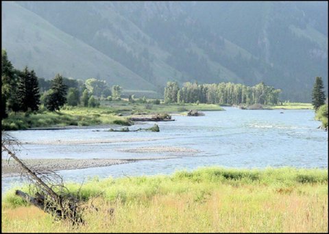
In the South Park area (from Jackson and Wilson to the narrowing of the valley 7 miles south), Love and Albee (1972) described the main aquifer: "Valley and stream deposits of gravel with lesser amounts of sand, silt, and clay. Surface is gravel underlain by thin discontinuous deposits of sand and silt." They mapped the remaining Quaternary alluvial deposits as "Flood-plain deposits; sand, silt, clay, and minor lenses of gravel; lesser amount of gravel at surface distinguishes these deposits." Nolan and Miller (1995) term the alluvial deposits occupying the main Snake River floodplain the "Jackson Aquifer" and provide geophysical evidence indicating the aquifer is between 380 feet (Antelope Flats area) and 2,400 feet (Potholes area) thick.
Water-well experience appears to bear out delineation of the Snake River alluvial aquifer within the larger body of Quaternary alluvial deposits. While prolific wells (transmissivities as high as 900,000 gpd/ft) are relatively common in the principal Snake River alluvial aquifer, wells in other areas of the alluvial aquifer are of more variable productivity and problems with sand production are not uncommon. The tested transmissivities of wells in the Rafter J and Melody Ranch areas (along Flat Creek south of Jackson), for example, are between 15,000 and 60,000 gpd/ft. These are still high-permeability deposits in the context of the surrounding bedrock geology, and are fully adequate for most non-agricultural applications, but are distinctly lower in permeability than in the coarser deposits along the Snake River.
"Other Quaternary Deposits" on Figure III-5 consist of a wide variety of glacial drift and outwash, loess, landslide debris and talus, swamp and lake deposits, talus breccia, conglomerate, and volcanic rocks. While these deposits are extraordinarily diverse in terms of their composition, they are grouped together here to reflect a generally lower groundwater production potential than the alluvial deposits discussed above. These deposits are also characterized by extreme heterogeniety. Particularly in deposits of glacial origin, highly-productive lenses of clean gravel may be present alongside dense clays with virtually no water-production potential. Loess deposits tend to be relatively unproductive of groundwater. Talus and landslide deposits, although quite permeable, tend to be relatively shallow and well-drained. Groundwater development in these non-alluvial deposits is best guided by detailed, site-specific investigations, for which the reader is referred to the bibliography and local experience.
In contrast to the Snake River alluvial aquifer, in many areas of the Salt River basin, the alluvium may be of substantial surficial extent, but is relatively thin, and successful wells have had to penetrate the underlying Salt Lake Formation. Contrary to the unfavorable descriptions of this formation provided by the USGS (Miller et al, 1996; Table 12), it has demonstrated quite variable water-bearing characteristics, both in terms of quantity and quality. For example, the spring system supplying the Town of Thayne issues from the Salt Lake Formation beneath a veneer of Quaternary-age alluvium. These springs are reported to flow 2,200 gpm, attributed to fracture enhanced permeability (Lines and Glass, 1975). Exploratory drilling west of this location (near the Town of Thayne) "encountered no significant water bearing formations", whereas a 310-ft. well nearer the springs was judged to be capable of 1,000 gpm (Forsgren Associates,1991).
Similarly, an exploratory well just west of Freedom encountered unacceptable groundwater quality in the Salt Lake Formation (total dissolved solids >1,000 mg/l), but a second well two miles east of Freedom had good quality and a yield of 650 gpm (Forsgren Associates,1991). Evaluation of Salt Lake Formation wells in the Alpine area found specific capacities (gpm per ft of drawdown) varied from over 10 to under 1 over distances of less than a mile. As with the Thayne springs, much of this was attributed to the influence of fracture systems (Sunrise, 1995).
Bedrock aquifers in the Snake/Salt River basin are mainly exposed in the upland areas. Tertiary-age rocks include volcanic deposits and a variety of conglomerate, sandstone, limestone, and mudstone sedimentary rocks. The productivity of these deposits with respect to groundwater varies locally, as a function of variations in texture, thickness, and fracturing. Successful development of useful water supplies, where possible at all, depends upon careful siting and exploration. For example, productive wells at Alpine and the spring system supplying Thayne both discharge water from the Tertiary-age Salt Lake Formation.
Mesozoic-age strata in the Snake/Salt River basin are dominated by thick shale formations. Productive wells have been developed locally from interbedded sandstone and conglomerate strata, but as a general rule these strata are relatively unproductive.
Paleozoic-age rocks consist primarily of thick limestone and sandstone formations. These include the Madison Limestone which is famous for producing high capacity groundwater wells at many Wyoming locations. As with all the other bedrock aquifers, however, the productivity of these strata can be quite site-specific, depending upon local enhancement of permeability through fracturing and variations in composition. Limestone, for example, is virtually impermeable in its native state of deposition. Given the faulting and folding of bedrock in the Snake/Salt River basin, however, and the ability of circulating groundwater to expand permeability through solution, limestone units provide very high groundwater production rates under locally favorable conditions.
Groundwater Circulation:
Hydrology textbooks commonly begin with a diagram of the "hydrologic cycle" that shows the constant passage of water between the atmosphere, the surface, and the subsurface. With the exception of the water associated with the original deposition of each geologic unit (termed "connate" water and generally of very poor quality), groundwater resources are a function of recharge from and discharge to the surface. Groundwater aquifers provide a large storage reservoir filled by infiltration of precipitation, snowmelt, and streamflow. Water moves through this "reservoir" as a function of groundwater elevation gradients and is "released" through discharge to springs, streams, and wells and though uptake and evapotranspiration by vegetation from the root zone. Groundwater quality is controlled by the solubility of the minerals with which it comes in contact as it travels from recharge to discharge and by its residence time in the subsurface. Thus, the surface and groundwater resource is one body of water, moving through the basin at widely different rates, but ultimately dependent upon the same fundamental sources.
As discussed above, groundwater recharge occurs primarily across the upland areas of the Snake/Salt River basin. Figure III-6 (from HA-539) presents this general pattern, which is the same in the northern portion of the study area, as evidenced by the losing and gaining reaches of specific streams. This same pattern is expressed by the general distribution of ephemeral/intermittent streams vs. perennial streams. The former are commonly indicative of surface water flow being lost to groundwater; the latter are sustained by the year-round discharge of groundwater to the stream.
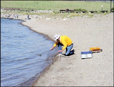
Combining groundwater gradients with permeability data for the alluvial aquifer, groundwater flow velocities on the order of 9 ft/day are indicated for the main Snake River alluvial aquifer (Jorgensen et al., 1999, p. 47). This is quite high, a reflection of the high permeability and abundant recharge to this aquifer. In the areas with a shallower and finer-grained alluvial aquifer and in bedrock aquifers, groundwater flow velocities are orders of magnitude slower. The time of travel from recharge to discharge of groundwater varies from days to years to decades to centuries to millenia, depending on the permeability, elevations, and distances involved (see Heath, 1983 for a general discussion).
Groundwater circulation is also influenced by seasonal and long-term fluctuations in groundwater levels. Figure III-7 presents those locations for which groundwater levels have been measured through the USGS monitoring program. In summary:
| Total number of sites | 308 |
| > 20 individual measurements | 13 (mostly from 1997/98 from the Jackson area) |
| 11 - 20 individual measurements | 19 (mostly from 1993/94 from Star Valley) |
| 3 - 10 individual measurements | 46 |
| 2 individual measurements | 48 |
| 1 individual measurement | 214 |
Those sites for which data have been collected over longer periods of time are most useful in the identification (and discrimination) of long-term and seasonal trends. Unfortunately, there are very few high-quality groundwater level monitoring data from the Snake/Salt River basin over any extended period of time. The most notable exception is the on-going research being conducted by the Wyoming State Engineer's Office in cooperation with Teton County in the "westbank" area (west of the Snake River, west of Jackson) as part of the "Jackson Hole, Wyoming, Environmental Restoration Feasibility Study".
Groundwater Development:
Geology
The geologic distribution of groundwater development is a function of the location of water demands and the availability of groundwater to meet those demands. Fortunately, in the case of the Snake/Salt River basin, these two factors are in rough coincidence, with the most productive aquifers occurring beneath the areas of highest demand, i.e. across the relatively gentle topography and private-land ownership of the floodplains of the Snake and Salt Rivers.
Use Trends
The primary development of groundwater in the Snake/Salt River basin is historically and currently for human consumption and related uses associated with domestic and municipal supplies (including subdivision, commercial, and other uses commonly permitted as "Miscellaneous"). Groundwater supplies the vast majority of these uses - approaching 100%. Although only a tiny proportion of total water use in the basin (approximately 8 % of that estimated for agriculture), this is arguably the most important water resource, as it directly sustains the human population.
From the companion technical memos of the Snake/Salt River Basin Plan, Table III-14 has been compiled:
Table III-14 - Groundwater Consumption in the Snake/Salt River Basin - 2002
| ac-
ft/yr | Notes |
Public Water
Supplies | 8000 | Average per capita “use” and population estimated for the 50 public water supplies in the study area (see Municipal Use Tech Memo), and assuming 50% consumption. |
| Rural Domestic | 1255 | (See Domestic Use Tech Memo) Assuming 50% consumption |
| Industrial
| <10
| (See Industrial Use Tech Memo) |
| Agricultural
| 650
| Compared with 99,000 acres under irrigation in the study area, there are only 603 acres with original-supply groundwater permits. At the average depletion rate calculated for irrigated acreage under the “wet year” scenario, the indicated groundwater depletion is 650 ac-ft, 86% of which is in the Salt River basin. |
The term "use" appears in many water studies without sufficient distinction between diversions/withdrawals and actual consumption (used up, removed from the local hydrologic system). Table III-14 presents estimates of groundwater consumption, with the understanding that actual withdrawals of groundwater necessary to sustain this consumption may be one or more times the listed quantities.
In the northern portion of the Snake/Salt River basin (i.e. the Jackson area), the great majority of this water is drawn from the alluvial aquifer along the Snake River, Flat Creek, and Fish Creek. In Star Valley, springs issuing from bedrock units (e.g. Madison Limestone, Bighorn Dolomite, Thaynes Limestone, and Twin Creek Limestone) along the east flank of the valley are the major source of groundwater developed by public water supplies. The Salt Lake Formation and the alluvial aquifer beneath the valley floor supplies local domestic wells and has seen substantial recent development to augment municipal supplies.
Table III-15 summarizes groundwater permit data for the Snake/Salt River basin. (The data for this and the remainder of this permit-based discussion comes from the electronic files of the WSEO, data entry current as of May 29, 2002.) Not surprisingly, domestic use dominates on a permit-count basis. Domestic, municipal, and miscellaneous uses, i.e. those representing human consumption, constitute 86% of the groundwater permits issued.
Table III-15 - Groundwater Permit Summary
| Use | Count | Average
Yield (gpm) | Average
Well Depth (ft) | Average
Water Level (ft) |
| Domestic | 3152 | 17 | 109 | 49 |
| Stock | 198 | 15 | 30 | 25 |
| Dom/Sto | 326 | 17 | 85 | 52 |
| Industrial | 7 | 110 | 92 | 44 |
| Irrigation | 71 | 367 | 123 | 34 |
| Misc. | 480 | 163 | 131 | 42 |
| Municipal | 18 | 692 | 206 | 51 |
|
Data from Wyoming State Engineer's Office files, current as of data entry on 5/29/02;
wells with inactive permit status and with zero yields excluded. |
Average well depths and average water levels reflect the relative abundance of developable shallow groundwater in the populated areas of the Snake/Salt River basin. The somewhat deeper average for municipal wells likely reflects the higher production requirements and the financial ability to penetrate more of the aquifer for additional protection from declining water levels and surface contamination.
Figure III-8 presents the temporal trend in groundwater development in the Snake/Salt River basin over the 20th century. From minimal development prior to the 1960's, groundwater permits have grown to over 4,000, with a cumulative permitted yield of 155,000 gpm. While this yield calculates to 250,000 ac-ft per year, the actual use of groundwater is far less. Few wells pump at their full permitted capacity more than a small percentage of the time. Following a decline in the pace of development in the mid-1980's, there have been 120 - 140 new domestic well permits issued each year throughout the 1990's. By county (within the Snake/Salt River basin) the last decade breaks down as:
| Teton County | 60 - 80 permits per year |
| Lincoln County | 45 - 55 permits per year |
| Sublette County | 6 - 8 permits per year |
The pace of stock, irrigation, and municipal groundwater development has remained relatively constant over the last 30 years, with an average of 6, 2, and 0.4 permits annually. The most recent permit issued for industrial groundwater use was in 1982. While this suggests no trend towards increased use, future groundwater development in this sector will be dependent upon the types of activity that may develop.
In summary, it is clear that the trend in groundwater development in the Snake/Salt River basin is dominated by additional, individual domestic wells. This trend is expected to continue as rural subdivisions proliferate in both the Jackson and Star Valley areas. Growth on the order of 100 to 150 wells per year are indicated, representing additional groundwater consumption on the order of 100 acre-ft per year.
Municipalities (and subdivisions with sufficient density to warrant central water systems) will continue to add incrementally to water supply facilities and will almost certainly continue to turn to groundwater. Current trends indicate 1 or 2 additional municipal supply wells in the basin each year. Consumption of groundwater associated with such wells will track municipal population growth.
Groundwater Levels
As noted above, there are relatively few data that address the issue of long-term changes in groundwater levels. Hydrographs for monitoring wells in the Snake/Salt River basin (see Figure III-7) show similar, regular seasonal changes in groundwater elevation over several annual cycles, with no overall up or down trend. We are aware of no areas within the Snake/Salt River basin where there has been a sustained change (increase or decrease) in groundwater levels over time.
Groundwater Quality:
Analyses
The primary source of groundwater quality data for the Snake/Salt River basin is the USGS, who have collected and analyzed samples from throughout the basin. Additional, site-specific data are commonly available from individual project reports (e.g. those of the WWDC) and from the files of water system operators. USGS water chemistry data by geologic unit in terms of total dissolved solids, and cations and anions for each unit can be found in the “Available Groundwater Determination” technical memorandum.
In the relatively open hydrogeologic system represented by the alluvial aquifers, recharge is rapid and aquifer residence times are relatively short. Thus, surface-derived water has little opportunity to become seriously mineralized. Existing water chemistry data demonstrate that total dissolved solids (TDS) concentrations are commonly less than 200 mg/l from these deposits and only rarely are above the EPA secondary drinking water standard of 500 mg/l. (Secondary standards are established with reference to color, taste, and general aesthetic quality rather than human health.) Much of the alluvial groundwater is relatively hard, likely the result of the abundance of limestone-derived sands and gravels. Where underlying bedrock formations make substantial contributions to the groundwater, as may occur along the deep faults bordering the east side of Star Valley and Jackson Hole, additional mineralization of groundwater may occur. Trace element and organics analysis of these waters suggests little need for concern, with the possible exception of iron and manganese which may locally exceed secondary drinking water standards.
As with the basic productivity of the bedrock aquifers, groundwater quality is quite variable. Due to the generally lower permeabilities and longer groundwater residence times, groundwater tends to be somewhat more mineralized than in the alluvial aquifer, although exceptions are not uncommon. Total dissolved solids concentrations over 300 mg/l are common from the Mesozoic aquifers; one well producing from the Mesozoic-age Bear River Formation with a TDS value over 1,000 mg/l. Trace element analyses demonstrate locally elevated levels of boron, iron, manganese, and zinc, again likely dependent upon site-specific conditions. The range of groundwater chemistry for the bedrock aquifers demonstrates that many are capable of yielding water supplies of acceptable quality. Site-specific conditions are of most importance in this regard, and those systems drawing groundwater from bedrock formations are the most likely to experience unacceptable concentrations of aquifer minerals.
Groundwater Contamination
Jorgensen et al. (1999) present a detailed discussion of potential groundwater contamination and wellhead protection for the developed portion of Teton County, including relevant ground
water quality standards and land use regulations and tables of groundwater contamination events. The following paragraphs are adapted and generalized from that report.
There are two general sources of potential contamination of groundwater supplies in the Snake/Salt River basin:
- 1) sources which affect broad areas, typically at relative low levels and over long time periods. Many of these are known as "non-point" sources and include septic system discharge and applications of agricultural chemicals like fertilizer, herbicides and pesticides.
- 2) localized discharges of contaminants, often at high concentrations, but in specific, limited areas. In the Snake/Salt River basin, these are generally limited to accidental spills and discharges. Both types of contamination are addressed under the general subject of wellhead protection - protection from contamination of the area through which groundwater flows to a water-supply well.
Figure III-9 depicts the density of domestic water wells in the Snake/Salt River basin by 40-acre tract, based on domestic well registration files of the Wyoming State Engineer's Office. (Groundwater permits are located only to the 1/4 1/4 Section.) Although aquifer contamination potential is a function of many local variables (e.g. depth-to-groundwater, permeability, aquifer thickness, aquifer lithology), a common "rule-of-thumb" is that domestic septic systems create potentially serious groundwater nitrate contamination problems at lot sizes of 2 acres or less. Assuming that each registered domestic-use well corresponds with a single-residence septic system, Figure III-9 provides a general picture of the density of potential nitrate sources. (2-acres lots correspond to 20 or more systems on a 40-acre tract.)
The spacing of individual wastewater septic systems is controlled by setback requirements with respect to water supply wells and septic systems and, perhaps most importantly, by minimum lot sizes in some areas. As an additional regulatory control on wastewater disposal contamination of groundwater, any subdivisions which have applied for county permitting after July 1, 1997 are subject to Wyoming Statute 18-5-306 which established the Subdivision Application Review Program within the Wyoming Department of Environmental Quality (WDEQ) - Water Quality Division. (See WDEQ, 1998.) Pursuant to this law, WDEQ has prepared guidelines to assess the adequacy of water and wastewater systems for all new subdivisions, and all new subdivisions are required to prepare engineering and hydrogeologic analyses of these systems. The required analysis includes investigation of groundwater contaminant loading by the proposed wastewater disposal system - whether a centralized facility or individual septic tanks and leach fields. The required area of investigation extends beyond the proposed subdivision to include the area through which groundwater will flow over a two-year time period.
The ease with which contamination may enter an aquifer is commonly termed the aquifer "sensitivity". It is primarily a function of the permeability distribution above and within the aquifer, the depth to groundwater, and the rate of recharge from the surface to the aquifer. As a general statement, the productive aquifers of the Snake/Salt River basin have a relatively high sensitivity to contamination because:
- High aquifer permeabilities allow rapid movement of contaminants between points of
recharge/infiltration and discharge.
- Permeable soils and the absence of low-permeability strata (e.g. confining layers)
between the surface the underlying aquifers allow surface contaminants to readily
reach groundwater.
- Depths to water are relatively small, allowing rapid transmission of surface contami-
nants to the water table.
- Aquifer recharge, particularly in areas subject to irrigation, provides the water to
carry contaminants into the groundwater system.
The University of Wyoming has recently completed a statewide assessment of groundwater vulnerability / aquifer sensitivity (Hamerlink and Arneson, 1998) based on general aquifer considerations. Their report includes a useful discussion of aquifer principles associated with sensitivity assessment; county-by-county appendices provide map details.
Figure III-10 presents a composite rating of aquifer sensitivity as developed by the University of Wyoming project. These ratings take into account generalized data on aquifer permeability, depth to the water table, the nature of the soils and other material above the water table, recharge rates, and land slope. Ratings have no absolute meaning; they simply reflect the relative sensitivity of the aquifer in one location as opposed to another. For perspective on these ratings, the area underlain by the main alluvial aquifer along the Snake River has received the highest possible sensitivity rating.
In summary, the developed aquifers of the Snake/Salt River basin are generally susceptible to aquifer contamination. Future planning and development should take this into account through appropriate site selection and design of water supply wells. In addition, the development of potentially conflicting uses in aquifer recharge areas should be monitored. Given the widespread use of the alluvial aquifer in the Snake/Salt River basin, individual "well-head protection plans" should be augmented with a general concern for all activities with potential for contamination of groundwater in and around the developable portions of the basin.
Groundwater Availability:
The "availability" of groundwater can be addressed in many ways, from calculation of the total groundwater present beneath a certain area or the total usefully recoverable groundwater present beneath a certain area (like a mineral resource), to calculation of the total annual groundwater output of an area (like streamflow), to calculation of the annual volume of groundwater that can be developed without significantly impacting other, existing water-resource users. The latter is the most appealing approach, but requires definition of "significant" and determination of which existing uses to consider (domestic, agricultural, environmental, aesthetic). The requirements of mass balance within any physical system ensure that any diversion of groundwater at one point results in an equal diminution of groundwater elsewhere, and that diminution must show up as a decrease in streamflow, evaporation, groundwater outflow from the system, evapotranspiration (crop, non-crop, human, animal), or groundwater storage.
The following paragraphs touch on each of these approaches in order to establish the general scale of the groundwater resource, but, as a practical matter, the availability of groundwater is a local and project-specific function of competing users, water quality needs, economics, and legal constraints, overlain upon the basic characteristics of aquifer properties and groundwater quality discussed above. Nonetheless, a few general conclusions can be made:
- The availability of groundwater across the Snake River alluvial deposits is physically limited only by the flow of the Snake River itself (3 million acre-ft per year). Aquifer permeability is sufficient, in most areas, to support production rates on the order of 1,000 gpm from individual wells. It is unlikely that groundwater development from this aquifer will impact surface flows sufficiently to trigger concerns about the volume of the combined water resource over any reasonable planning horizon. "Local water supplies are, in most cases, readily available through groundwater development. While each water supply system presents unique hydrogeologic and engineering concerns, the need for long-distance conveyance of water from areas of supply to areas of use is relatively unlikely" (Jorgensen et al., 1999). A more likely constraint on groundwater development in this area is the incremental deterioration of groundwater quality that accompanies the establishment of increasing domestic, municipal, commercial, and other uses.
- In Star Valley, the alluvial aquifer is of much less thickness than along the Snake River and is above the groundwater table in many areas. Successful well development across the valley floor has been primarily based on the highly variable Salt Lake Formation. Development experience with this formation demonstrates that high-volume wells are possible, but that careful, site-specific exploration is necessary and that groundwater of adequate quantity and quality may not be available at all sites.
Springs issuing from bedrock units on the east side of Star Valley have been extensively developed and, with adequate safeguards with respect to water quality, can be expected to continue.
- Bedrock aquifers in upland areas provide a full spectrum of groundwater development potential, from low permeability and low quality to highly productive aquifers with good water quality. Due to the complexities of the study area bedrock geology, these conditions are quite site-specific and can change dramatically over short distances. Detailed, site-specific evaluations and exploratory drilling should be anticipated in areas where groundwater is anticipated from these units.
Basically, subsurface materials are saturated with water from the water table, a relatively short distance below land surface in most areas, to the depth at which there is no significant porosity to contain groundwater, e.g. the crystalline basement rocks underlying the entire Snake/Salt River basin and forming the visible core of the highest mountains. The volume of pore space in this material represents the volume of groundwater and is likely on the order of 100's of millions of acre-ft. Much of this water is of unusable quality (e.g. due to great depth) or is contained in formations from which groundwater cannot be extracted at useful rates (e.g. thick shale units), so the useable groundwater resource is vastly smaller than the total groundwater in storage.
Considering only the alluvial aquifer (covering approximately 400 mi2) in the Snake/Salt River basin, and assuming an average saturated thickness of 200 feet and an effective porosity of 20%, a volume of 10 million acre-ft of useful groundwater in storage is calculated. Were groundwater a static, nonrenewable resource, like coal, this volume might approximate the developable resource.
Groundwater is very dynamic resource, however, particularly groundwater of high quality occurring at depths feasible for development. Data suggest an average annual recharge rate of approximately 4 inches = 1 million ac-ft/yr spread across the 4700 mi2 of the Snake/Salt River basin. The base flows of the Salt and Greys Rivers (i.e. the streamflow that is sustained by groundwater input through the period of the year without significiant precipitation input) suggest average groundwater output of 250 and 350 ac-ft/mi2/yr, respectively. (The Snake River basin below Jackson Lake is not considered due to the impact of reservoir modulation on base flows.) Applying a value of 300 ac-ft/mi2/yr to the entire basin suggests a total groundwater output of 1.5 million ac-ft/yr, roughly comparable to the recharge-based estimate. Of course, development and consumption of this "available" groundwater would leave the streams of the Snake/Salt River basin dry through much of the year.
A more detailed, groundwater-model based mass balance for the alluvial aquifer between Jackson Lake and Hoback Junction was developed by San Juan and Kolm (1996). They estimated total recharge of approximately 50,000 acre-ft per year, with 25,000 acre-ft per year of groundwater discharge through evapotranspiration and 25,000 acre-ft per year of discharge to streams.
In any case, the inescapable requirements of mass balance mean that additional groundwater consumption causes either a decrease in groundwater storage (declining groundwater level/pressure), a decrease in consumption elsewhere in the hydrologic system, or depletion of surface water. As discussed above, there is little indication of widespread reductions in groundwater levels in the study area (although long-term data are sparse).
Geothermal Resources:
For certain applications, the temperature of groundwater may itself be a useful resource. Thermal energy can be usefully extracted from groundwater at temperatures as low as 40°F through the use of groundwater heat pumps, typically used for small space-heating loads. For small-scale, e.g. residential, applications of this level of geothermal energy, little is required beyond a sustainable source of groundwater on the order of a few gallons per minute. At the opposite extreme of geothermal resources are natural occurrences of super-heated steam which can be tapped to drive electrical generators. Such occurrences are quite rare and require special circumstances of heat sources and groundwater circulation. In between are a wide variety of geothermal applications, including spas, swimming pools, commercial space heating, de-icing systems, fish propagation, hydroponics, industrial process heating, district space heating, and generation through the use of binary fluid systems.
Most of the geothermal resources in Wyoming are a function of the deep circulation of groundwater. The natural "plumbing" of an aquifer carries recharge water sufficiently deep to be significantly heated by the normal geothermal gradient of the earth - approximately 14°F per 1,000 feet of depth. Groundwater circulation (or deep drilling) then brings this water sufficiently close to the surface that it can be economically developed for moderate-temperature, near-source applications. Only in the Yellowstone National Park area are there special subsurface sources of heat that produce very hot groundwater and even super-heated steam.
Occurrence
Although not hosting the extensive, deep sedimentary basin type of geothermal resources that are present elsewhere in Wyoming, the Snake/Salt River basin has a variety of local geothermal features. These vary from the 64°F flow of the Teton Valley Warm Springs near Kelly, to 200°F thermal springs in the Yellowstone Park portion of the basin. Geochemical indicators suggest a subsurface temperature of 270°F for the Huckleberry Hot Spring system, just south of Yellowstone, but this likely marks the southern extent of the Yellowstone geothermal system that draws its heat from a cooling body of molten rock at depth. South of Yellowstone, geothermal features are generally of lesser temperature and are largely a function of deep groundwater circulation along local fault systems. There is no concentration of geothermal features in the Snake/Salt River basin, but isolated occurrences in both valley and upland settings.
The only exception to this generally moderate-grade resource of which we are aware is at the Auburn Hot Springs. This is the only geothermal system in Wyoming outside Yellowstone (and the Huckleberry Hot Springs area immediately south of Yellowstone) where geochemical indicators suggest subsurface temperatures (300°F) potentially high enough to approach electrical generation potential. The surface discharge of this system has a maximum temperature of approximately 140°F.
Development
Due to its location primarily within the national park, the Yellowstone geothermal system has been developed only in terms of its scenic and aesthetic values, and scientific research has been focused on geological and biological processes rather than on the resource's commercial potential. (Prospecting with regard to exotic, high-temperature microbes may represent an exception.) Elsewhere in the basin, land ownership patterns also impact the potential development of geothermal resources, with several local systems falling within other National Park and National Forest lands. While several of these features host recreational use (e.g. Huckleberry Hot Springs, Granite Hot Springs) and thermal springs at the Jackson Fish Hatchery are used in fish-rearing operations, there is little likelihood of more intense development.
Geothermal features on non-federal and private lands are similarly used primarily simply as attractive sources of warm water for bathing, swimming, soaking, limited low-technology space heating, and, in the case of the Kelly Warm Springs, for kayak practice sessions.
Despite the limitations on geothermal development imposed by land ownership patterns in the Snake/Salt River basin, there are scattered occurrences of local geothermal systems with development potential for moderate-temperature applications. If the present understanding of these systems as largely fault controlled is correct, there is potential for increased development through drilling - an improvement in volume, reliability and control over simply taking the natural flow of warm springs. However, that potential is likely localized along the controlling geologic structures and the potential for subsurface temperatures substantially higher than the observed discharge temperatures (rarely >110°F) is small.
To date, development interest and economics have not justified applications much beyond the obvious pleasures of direct contact with warm water. The most viable candidate for development appears to be the system at Auburn, which is largely located on private lands. However, intermittent exploration interest over many decades has so far been unsuccessful in identifying an economically viable application.
E. WATER CONSERVATION
Introduction:
Water conservation in the Snake/Salt River basin involves all uses including agriculture, municipalities, industry, recreational, and environmental concerns. In the past, water conservation efforts were mainly focused on improving efficiency of agricultural water use. As communities within this basin have changed, there is a growing interest in flat water activities and stream flow related recreation. The following is an examination of water conservation activities and opportunities in the Snake/Salt River basin.
Agricultural Water Conservation:
Flood irrigation utilizing canals and ditches was the standard method of distributing irrigation water until the late 1960's and early 1970's. At that time, many areas of the Salt River basin converted from flood irrigation methods to pressure irrigation using sprinklers. This provided a much more efficient way of supplying water to the growing plants, and greatly reduced the quantity of water lost during conveyance as well as seepage losses from over-application of water. As the efficiency of water distribution increased, the reduced flows in late summer could be applied to a larger area, thus increasing yields. However, the reduction in conveyance and seepage losses also resulted in less water to recharge the groundwater system, and return flows in the fall and winter were reduced. Another result was that spring runoff that had been previously diverted and flooded in the fields was now allowed to stay in the stream, which resulted in higher peak flows during runoff.
The topic of change in agricultural production due to the conversion to sprinkler irrigation has been discussed with local producers. According to one producer in the Salt River basin, when utilizing flood irrigation he would produce approximately one ton of alfalfa per acre per year, and 34 bushels of barley per acre per year. Rarely did they have enough hay growth for a second crop. After the installation of sprinkler irrigation, yields increased to over 4 tons of alfalfa per acre per year, and 95 bushels of barley per acre per year. While previously the farm could support about 25 dairy cows and was short of hay on some years, they now have adequate feed for 50 cows utilizing the same farm ground. The improvement caused by sprinkler irrigation is seen in more than just crop yields. It was estimated that 10% of the farm ground was used for ditches and laterals, where now most of this ground is now used for growing crops due to the elimination of ditches within the field as well as the installation of buried pipe. Also, harvesting has become much more efficient without having to cut around the various distribution laterals and ditches in a field.
Municipal and Industrial Water Conservation:
Water conservation measures have been implemented by some of the municipalities in the basin, however it has not been a major focus. The largest town in the basin, Jackson, has implemented metering as have many other public water systems. However, many public systems do not meter their water use and have no incentive to conserve water. The expense of installing meters can be seen as prohibitive, and is unpopular politically. Also, some systems encourage water use during the winter months to prevent frozen pipes. Some systems are requiring meters on new hookups, and look to phasing in metering to the existing population.
During the last two summers, drought conditions have prompted some communities, such as Afton, to implement voluntary and mandatory water restrictions. Generally, these restrictions have consisted of elimination of outside lawn watering during daytime hours with exceptions for automatic sprinkler systems. In Afton, this was done to reduce daytime demand to better match the output from the Periodic Spring.
Recreational and Environmental Water Conservation:
Various wetland and riparian enhancement projects have been conducted throughout the basin over the years. While these projects do not necessarily conserve water, they do conserve or enhance habitat for fish, waterfowl, and other animals. Also, maintenance flows at the Jackson Lake Dam have been agreed to by the U.S. Bureau of Reclamation in order to provide sufficient flow in the Snake River for fish during the winter months.
Future Conservation Opportunities:
In general, the Snake/Salt River basin has adequate water to serve the needs of basin residents. For the most part, water shortages are seasonal, and their effects can be magnified by drought conditions. In spite of the adequate availability of water, and perhaps because of it, conservation methods can be used in virtually every form of water use.
Agricultural Conservation Opportunities
The largest water savings by quantity are generally realized by conservation in the agricultural sector, as it represents the largest use of water in the basin. For this reason, much of the focus of water conservation is on irrigation practices. In order to determine what future conservation efforts will be effective, an inventory of existing facilities is necessary. Major items of interest in this inventory include conveyance facilities and irrigation methods. A summary of this data is presented in Table V-3. Only major irrigation diversions with adequate accompanying data were included. Roughly 60 percent of the irrigated land in the entire Snake/Salt River basin is included in these calculations.
Table V-3. Major Ditch Conveyance and Irrigation Methods Summary
| Sub-basin | Canal
(miles) | Pipe
(miles) | Irrigated
Acreage | % Flood
Irrigated | % Sprinkler
Irrigated | Acres Flood
Irrigated | Acres Sprinkler
Irrigated |
| Upper Salt River | 29.0 | 54.0 | 19,239 | 32.4 | 67.6 | 6,237 | 13,002 |
| Lower Salt River | 54.5 | 22.5 | 17,210 | 17.8 | 82.2 | 3,070 | 14,140 |
| Upper Snake River | 6.6 | 0.0 | 2,927 | 100.0 | 0.0 | 2,927 | 0 |
| Lower Snake River | 62.5 | 3.8 | 14,160 | 97.7 | 2.3 | 13,830 | 331 |
| Teton River | 18.9 | 0.0 | 8,742 | 0.0 | 100.0 | 0 | 8,742 |
| Total= | 171.5 | 80.3 | 62,278 | 41.8 | 58.2 | 26,063 | 36,215 |
|
A significant portion of water diverted for irrigation can be lost during conveyance to the field through seepage, deep percolation, phreatophytes, evaporation, and so forth. Water is typically diverted from the river or stream into a canal or ditch, which is generally of earth construction and unlined. The soils in the Snake/Salt River basin are predominantly gravelly loams as they were formed on the alluvium of the many rivers, streams, and washes that are present in the valleys. Naturally, water will quickly percolate through these granular soils. Essentially none of the canals and ditches in the basin are lined, yet many have been somewhat sealed over time with the deposition of fine material. Losses though unlined canals and ditches have been estimated at up to 40 percent of the diverted flow, however there are no extensive studies that have evaluated ditch conveyance losses in the Snake/Salt River basin.
Irrigation methods also present an opportunity for water conservation. In the Snake/Salt River basin, historically flood irrigation was the most popular method used in spite of its low efficiency. However, since the early 1970's many areas, particularly in the Salt River basin, have converted to sprinkler irrigation that utilize hand lines or wheel lines. There are a few isolated areas that have incorporated center pivot irrigation. For the most part, the conversion from flood to sprinkler irrigation has had a positive effect, as crop yields have increased considerably. Also, more acres of cropland can be irrigated late in the summer when there is less water available. However, some positive aspects of flood irrigation have been reduced with the conversion to sprinkler, such as groundwater recharge and delay of the peak runoff.
Municipal Conservation Opportunities
Municipal water use is the next significant use of water in the basin following agricultural water use. Conservation measures for these types of systems generally consist of individual customer meters that track actual water use. Meters can also help determine if there are major losses in the distribution system through leaks. Some municipal water systems have implemented water restrictions, both voluntary and mandatory, during the summer over the past two years of drought. These restrictions effected irrigation of lawns and landscaping during high use times, and encouraged the use of automatic sprinkler systems. Conservation efforts on municipal systems have been shown to reduce indoor use by over 20 gallons per capita per day. Outdoor water use for irrigation of lawns and landscaping can be significant, and can be greatly reduced by utilizing plants with lower water requirements and installing sprinkler systems and timers. Perhaps the largest municipal or domestic use of water is sprinklers and hoses left running around the clock during the summer. Also, due to water systems that are shallow and subject to frost, many communities encourage water use such as running a constant stream of water in the winter to prevent frozen pipes.
Recreation and Environmental Conservation Opportunities
Much of the use of water in the Snake/Salt River basin is related to recreational and environmental uses. While these are generally non-consumptive uses, water is still key to many of these activities. Conservation efforts in these areas generally do not conserve the quantity of water used, but rather focus on conservation of a fishery, wetland, or other resource that serves to improve the water use opportunity. Water storage can serve an important role in meeting these water needs by providing increased management of the available water supply for these uses. Storage can also serve to conserve water by meeting the needs of the resource while holding over surplus water for later use. For another example, fencing to keep cattle off of a stream bank can help reduce erosion, improve water quality, and maintain habitat. In these circumstances, an off-stream location for stock watering must be developed. Without an alternative water source, fencing may also mean that an irrigated crop, either by natural or artificial means, may not be harvested or grazed. Also, water utilized for wetlands may be considered conservation of bird or fish habitat, although more water is used than if the wetland was not maintained.
Conclusion:
In order for conservation methods to be successfully implemented, there must often be an incentive or benefit for those involved. This incentive may be in various forms, such as increased crop yields, improved fishing, reduced costs, and so forth. Reduction of conveyance losses and improvement of irrigation efficiency does not necessarily equate to less water used. In areas of deficit, conservation measures may result in the conserved water being applied to additional acres or providing a full supply of water throughout the season without a decrease in the water diverted. However, this improvement in efficiency will likely result in an increase in the crop quality and yield. Prior to implementation of conservation improvements, the system should be studied to see how conservation is addressing the issue and to make sure that the program will have the intended result.
Figure III-3: Snake River Node Diagram
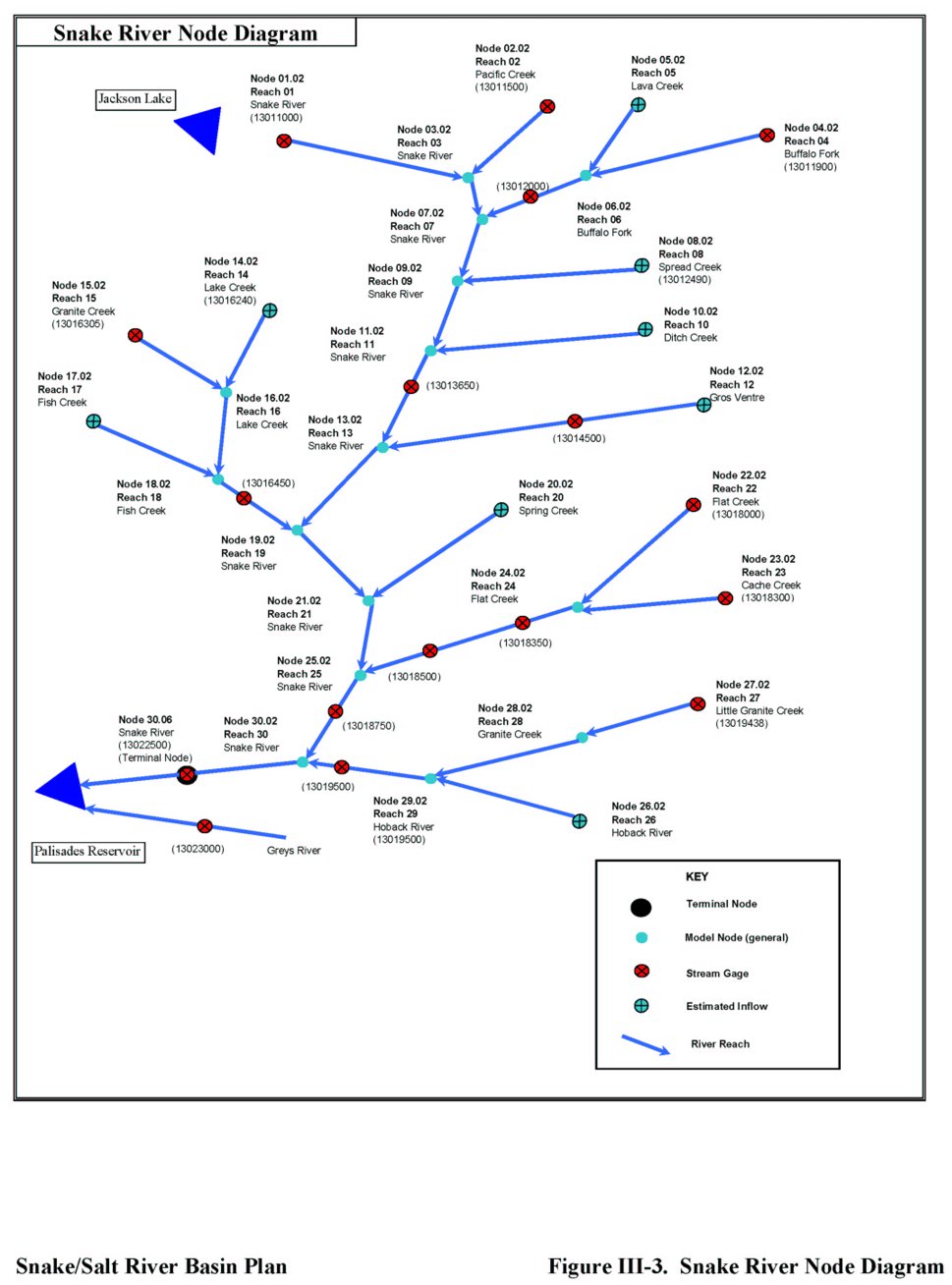
Figure III-4: Salt River Node Diagram
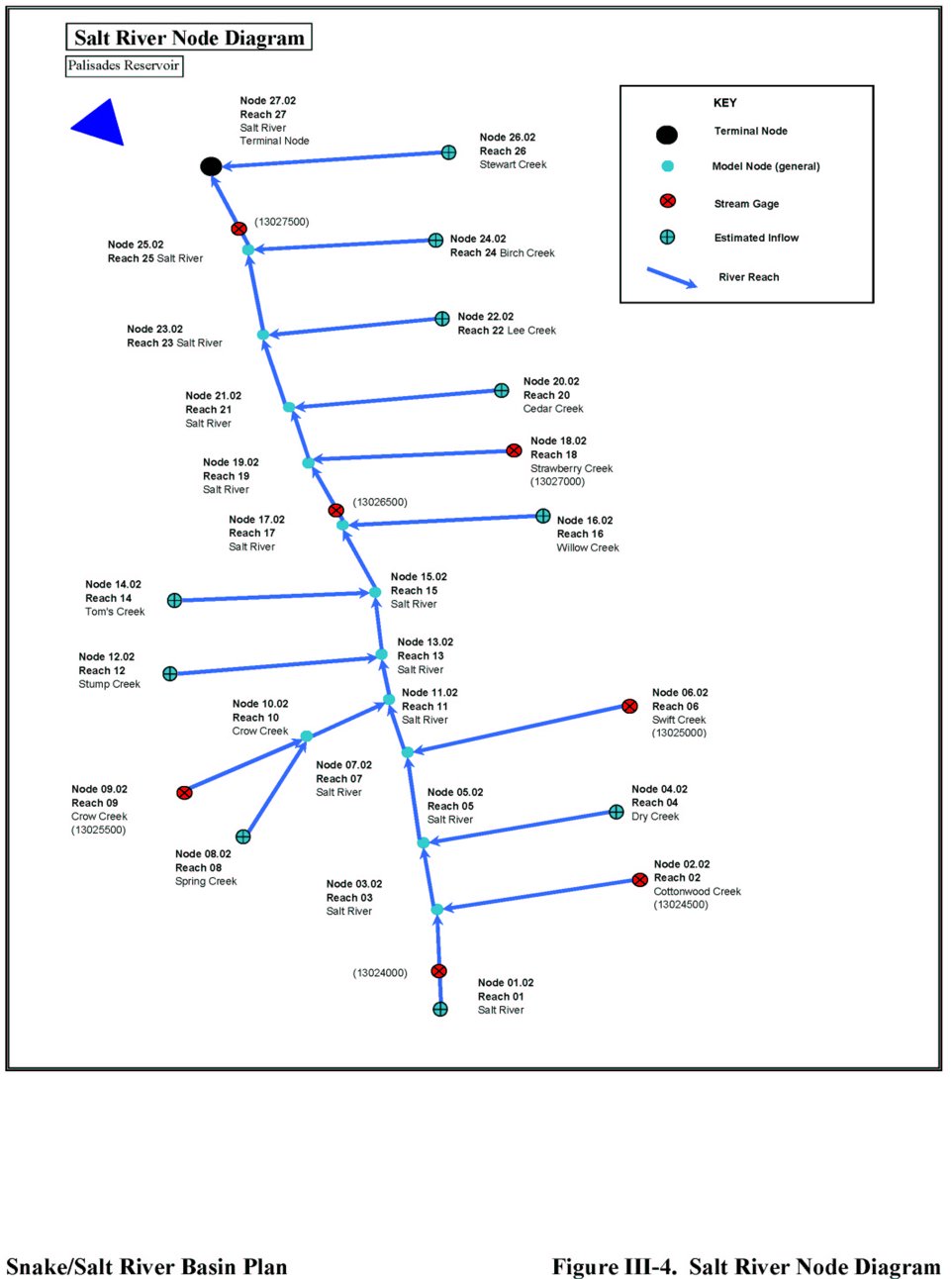
Figure III-5: General Geology and Well Density
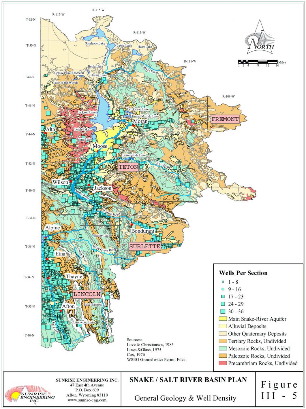
Figure III-6: Shallow Aquifer Recharge Rates
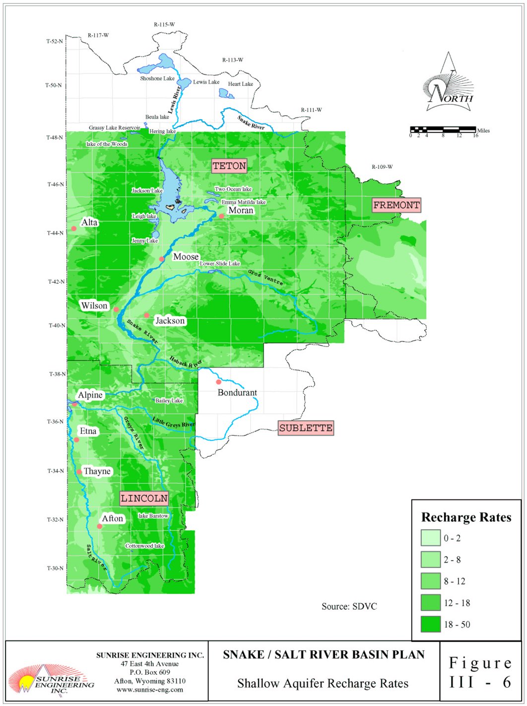
Figure III-7: USGS Ground Water Elevation Monitoring Sites
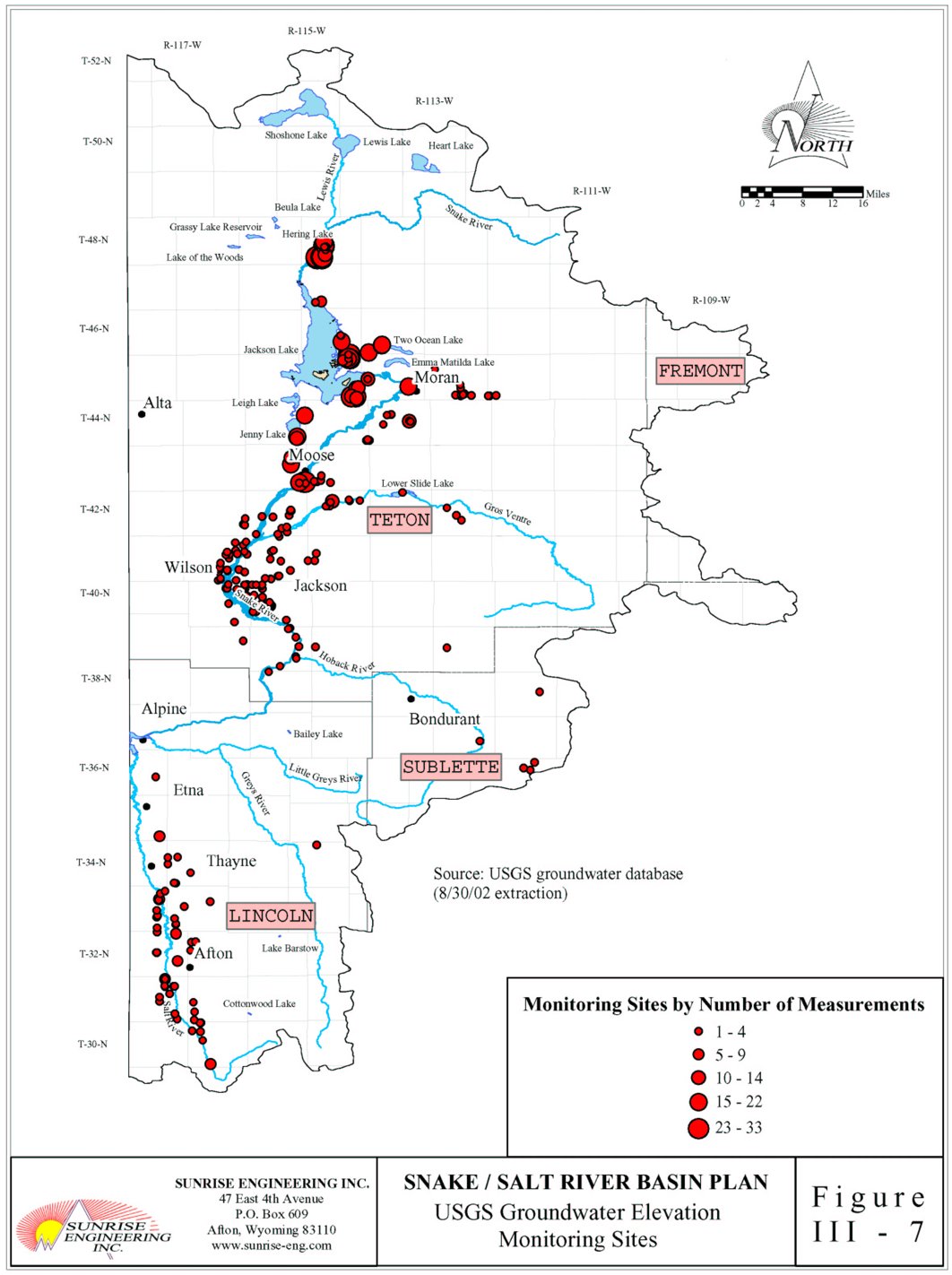
Figure III-8: Ground Water Permits for Domestic Use by Decade
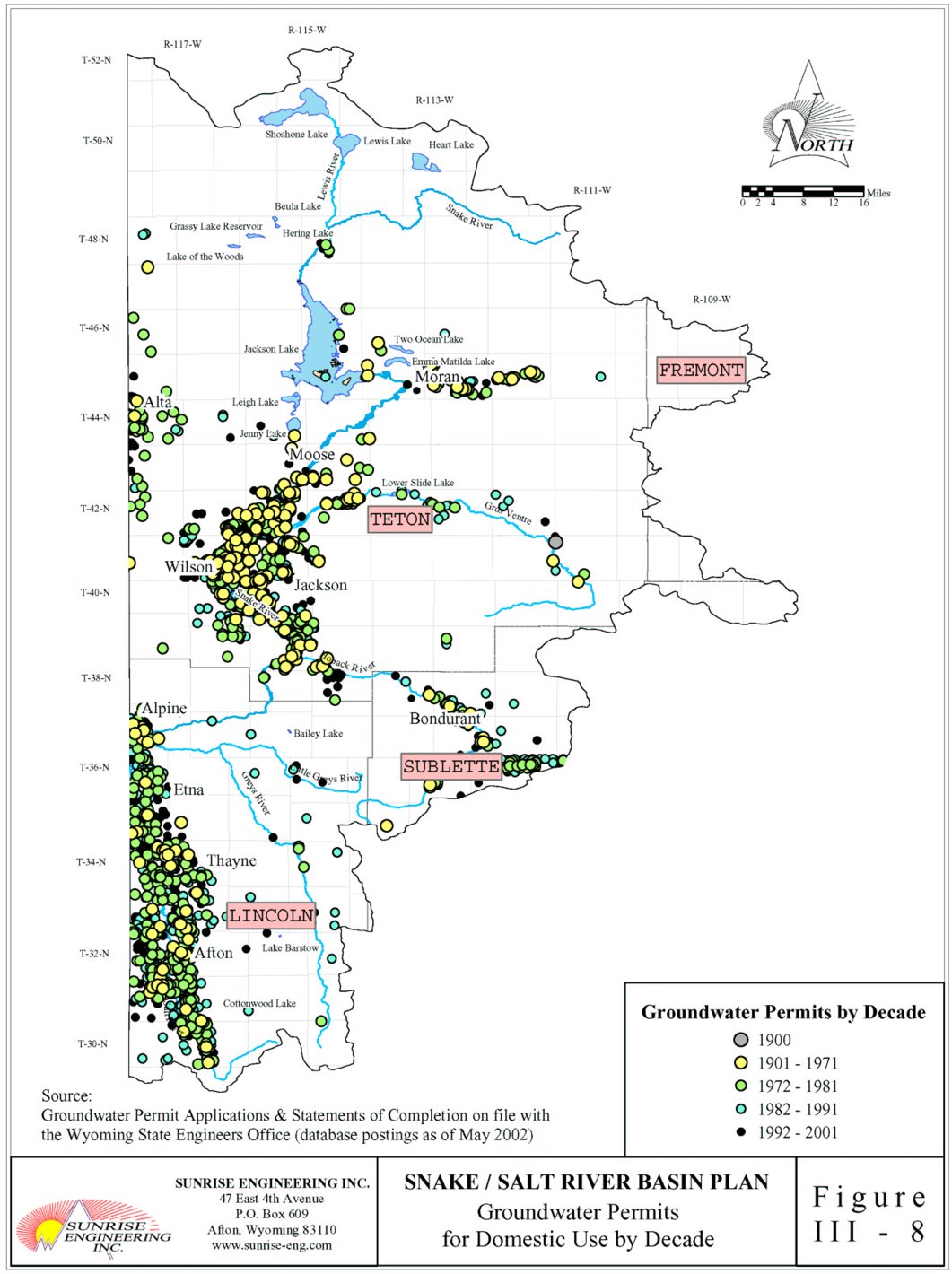
Figure III-9: Wyoming State Engineer’s Office Permit Locations
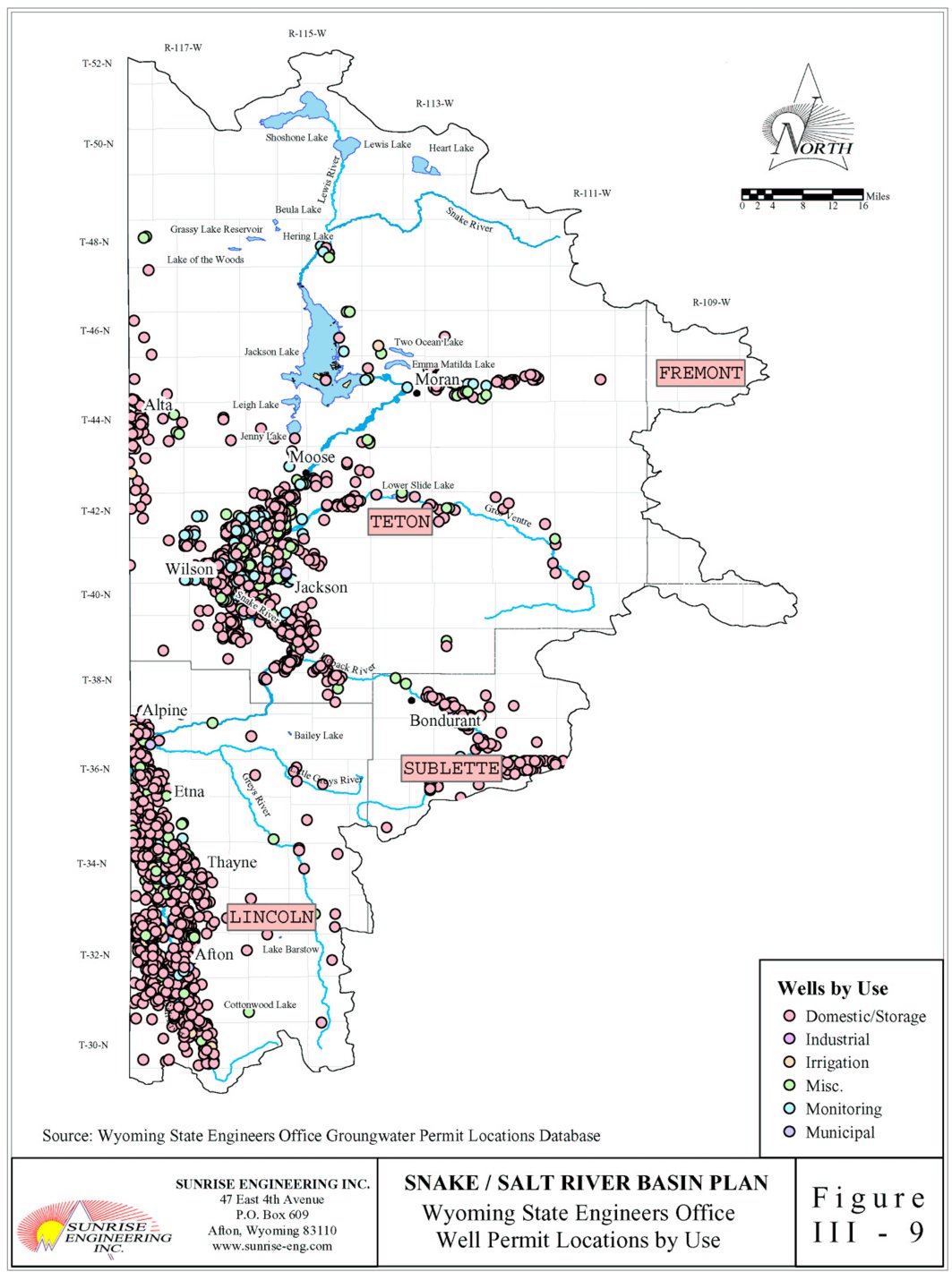
Figure III-10: Aquifer Sensitivity