Wyoming State Water Plan
Wyoming State Water Plan
Wyoming Water Development Office
6920 Yellowtail Rd
Cheyenne, WY 82002
Phone: 307-777-7626

Wyoming Water Development Office
6920 Yellowtail Rd
Cheyenne, WY 82002
Phone: 307-777-7626

TECHNICAL MEMORANDUM
Introduction
The Wyoming Water Development Commission (WWDC) has undertaken water basin planning efforts throughout Wyoming. The purpose of the statewide planning process is to provide decision-makers with current, defensible data to allow them to manage water resources for the benefit of all the state’s citizens. Under Tasks 3B and 3C, spreadsheet models were developed to determine average monthly streamflow in the basin during normal, wet, and dry years. The purpose of these models was to validate existing basin uses, assist in determining the timing and location of water available for future development, and help to assess impacts of future water supply alternatives.
The WWDC specified that the models developed for the various Wyoming river basins be consistent, and use software available to the average citizen. Accordingly, Excel was selected as the platform to support the spreadsheet modeling effort . The spreadsheet model developed for the Bear River, the first basin plan undertaken, became a template for subsequent river basin modeling, and new features were added as unique circumstances were encountered in those basins. In this task, the spreadsheet models used in the Powder/Tongue River Basin Plan were used as a basis and were re-populated with Salt and Snake River node networks and associated data. The existing logic was adequate to express operations in these two basins, and there were no substantial changes to the spreadsheet logic.
Tasks 3B and 3C encompassed creating and calibrating six spreadsheet workbooks, one for each of three hydrologic conditions and two distinct sub-basins:
The three workbooks for each sub-basin are yoked together with a simple menu-driven graphical user interface (GUI), effectively creating two sub-basin models.
Scope and Organization of this Memorandum
This memorandum is intended to be both a user’s guide and engineering documentation of the models. After a section describing the models in general terms, the document’s organization follows the organization of worksheets in the model. The subsection “Model structure and components” describes the types of worksheets and the format of the worksheet documentation that follows. Engineering details of particular length or complexity have been placed in appendices, with “pointers” to them in the appropriate worksheet descriptions. The remainder of this memorandum comprises the following sections and subsections:
Spreadsheet Models
Model overview
Model development
Model structure and components
The Navigation Worksheets
The central navigation worksheet
The basin map
The results navigator
The Input Worksheets
Master List of Nodes
Gage data
Diversion data
The Computation Worksheets
Reach gain/loss
The Reach/Node Worksheets
Snake River notes
Salt River notes
The Results Worksheets
Outflows
Diversions
Model Overview
For each Snake/Salt River sub-basin, three models were developed, reflecting each of three hydrologic conditions: dry, normal, and wet year water supply. The spreadsheets each represent one calendar year of flows, on a monthly time step. The modelers relied on historical gage data from 1971 to 2001 to identify the hydrologic conditions for each year in the study period, as discussed in the technical memorandum for Task 3A Surface Water Data Collection and Study Period Selection. Because historical diversion data were virtually unavailable for this period, total diversions and resulting return flows were not explicitly included in the spreadsheets. Instead, only the consumptive portion of diversions is taken out of the stream in the models. Thus, streamflow and consumptive use are the basic input data to the model. For these data, average values drawn from the dry, normal, or wet subset of the study period were computed for use in the spreadsheets. The models do not explicitly account for water rights, appropriations, or compact allocations nor is the model operated based on these legal constraints. It is assumed that the limitations that may be placed on users due to water rights restrictions are reflected in the number of irrigating days included in the consumptive use calculations for each of the three hydrologic conditions.
To mathematically represent each sub-basin system, the river system was divided into reaches based primarily upon the location of major tributary confluences. Each reach was then sub-divided by identifying a series of individual nodes representing diversions, tributary confluences, gages, or other significant water resources features. The resulting network is the simplification of the real world that the model represents. Figure 1 and Figure 2 present node diagrams of the models developed for the Snake and Salt River sub-basins. The numbered nodes in the diagram represent primarily gage or inflow nodes and confluence nodes; the diagram does not depict diversion nodes.
Virgin flow for each month is supplied to the model by specifying flow at every headwater node, and incremental stream gains and losses within each downstream reach. Where available, upper basin gages were selected as headwater nodes; in their absence, flow at the ungaged headwater point was estimated outside the spreadsheet. For each reach, incremental stream gains (e.g., ungaged tributaries, groundwater inflow, and inflow resulting from human-caused but unmodeled processes) and losses (e.g. seepage, evaporation, and unspecified diversions) are computed by the spreadsheet. These are calculated by adding net modeled effects (diversions) within the reach back into the difference between the upstream and downstream historical gage flows. Stream gains are input at a point in the reach below the gaged or estimated inflow to be available for diversion downstream and losses are subtracted at the bottom of each reach.
At each node, a water budget computation is completed to determine the amount of water that flows downstream out of the node. The amount of flow available to the next node downstream is the difference between inflow, including upstream inflows, return flows, imports and reach gains, and outflows, including diversions, reach losses and exports. For the Snake/Salt Rivers, imports/exports and return flows are not modeled explicitly, but are set to zero in the water budget calculation. Diverted amounts at diversion nodes are the minimum of demand (consumptive use requirements) and physically available streamflow. Mass balance, or water budget, calculations are repeated for all nodes in a reach.
Model output includes the diversion demand and simulated diversions at each of the diversion points, and streamflow at each of the Snake/Salt River Basin nodes. Impacts associated with various water projects can be estimated by changing input data, as decreases in available streamflow or as changes to diversions occur. New storage projects that alter the timing of streamflows or shortages may also be evaluated.
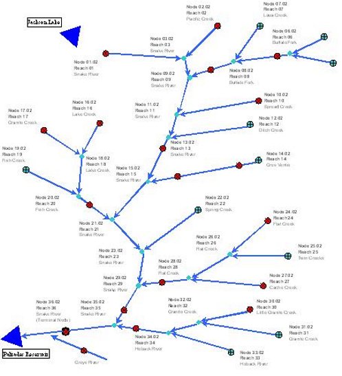
Figure 1 Snake River Node Diagram
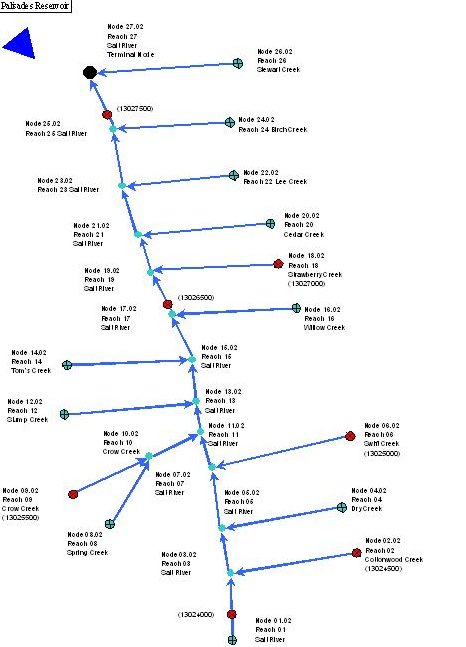
Figure 2 Salt River Node Diagram
Model Development
The model was developed using Microsoft® Excel 97 and Excel 2000. The workbooks contain macros written in Microsoft® Excel Visual Basic programming language. The primary function of the macros is to facilitate navigation within the workbook. There are no macros that need to be executed to complete computation of any formulas or results. In other words, whenever a number is input into any cell anywhere in the workbook, the entire workbook is recalculated and updated automatically.
The model was developed with the novice Excel user in mind and it is assumed that the User has a basic level of proficiency in spreadsheet usage. Every effort has been taken to lead the User through the model with interactive buttons and mouse-driven options. This memorandum will not provide instructions in the use of Excel for this spreadsheet.
Model Structure and Components
Each of the Snake/Salt River sub-basin models is a workbook consisting of numerous individual pages (worksheets). Each worksheet is a component of the model and completes a specific task required for execution of the model. There are five basic types of worksheets:
In the following sections, each component of the Snake/Salt River Basin Models is discussed in greater detail. A general discussion of each component includes a brief overview of the function. The discussion of each component also generally includes two sections:
Engineering Notes: Detailed discussion of methodologies, assumptions, and sources used in the development of that component; andUser Notes: “How to” instructions for model Users.
Programmer Notes, which are instructions and suggestions for programmers modifying the model, are included in Appendix A. These will assist state staff with any modifications of this model to analyze changed conditions or other applications in the Snake/Salt River Basin. Additionally, since this model may be a basis for developing spreadsheet models for other basins, this will serve as a guide for other consultants.
The Navigation Worksheets
A GUI was developed to assist the User in navigating the sub-basin workbooks. The top-level navigation sheet is initialized by opening the appropriate Snake/Salt River Basin Model Excel file:
The GUI provides a brief tutorial and information regarding the current model version (Figure 3). From the GUI, the User may select the dry, normal, or wet year model.
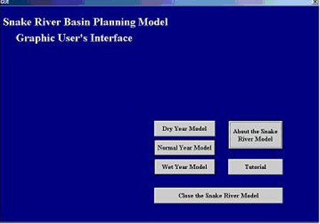
Figure 3 Graphical User’s Interface for the Snake River Model
User Notes:Upon opening the Snake or Salt River file, the User is presented with several options:
Dry Year Model: Open the Dry Year Model workbook,
Normal Year Model: Open the Normal Year Model workbook,
Wet Year Model: Open the Wet Year Model workbook,
About the (Sub-basin) Model: Obtain information pertaining to the current version of the model,
Tutorial: Open a brief tutorial that describes the general structure of a spreadsheet workbook
Close the (Sub-basin) Model: Close any open workbooks.
The Dry, Normal, and Wet Year models each have two main navigation worksheets to view other portions of the workbook. A third sheet contains a diagram of the basin to orient the user, and also contains links directing the User to reach calculation worksheets. For Users experienced with Excel spreadsheets, all conventional spreadsheet navigation commands are still operative (e.g., page down, GOTO, etc.).
The Central Navigation Worksheet
The Central Navigation Worksheet is the “heart” of the model. From here, the User can “jump” to and from any worksheet in the model. Figure 4 displays the Central Navigation Worksheet from the Salt River Basin Normal Year Model.
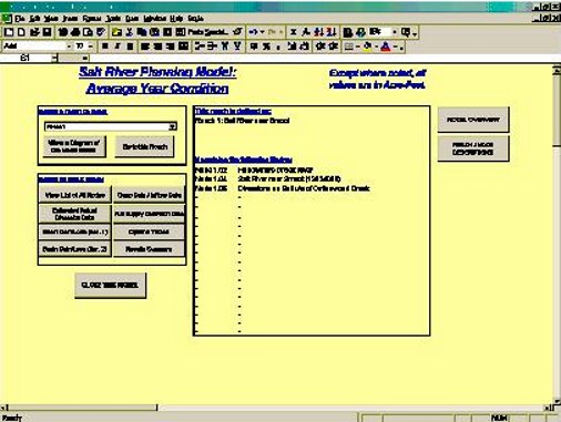
Figure 4 Central Navigation Worksheet for the Salt River Planning Model:
Normal Year Condition
User Notes:This is the first worksheet the User sees upon selecting a hydrologic condition from the GUI. Using the gray buttons, the User can “jump” to
- the basin diagram (View a Diagram of the Model Nodes),
- any of the Reach/Node worksheets (Go to this Reach),
- the Input Worksheets and Computation Worksheets (Estimated Actual Diversion Data, Basin Gain/Loss, Gage Data/Inflow Data, View List of all Nodes), and
- the Results Navigator (Results Summary) which leads in turn to several summaries of output.
The User specifies the reach he wants to go to by selecting it from the pull-down menu. When a reach is selected, the table to the right lists all the nodes in that reach by number and name.
The Basin Map
User Notes The Basin Map Worksheet provides a simple “stick diagram” of the basin. The User can navigate to a specific reach worksheet by clicking on an object on the diagram.
The Results Navigator
User Notes
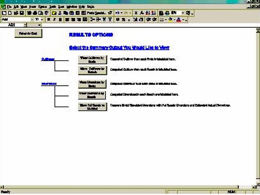
Figure 5 Results Navigator
The Results Navigator (Figure 5) allows selection of any of the following output tabulations:
- Outflows summarized by reach
- Outflows summarized by node
- Diversions summarized by node
- Diversions summarized by reach
- Modeled versus estimated or historical diversions
The Input Worksheets
Master List of Nodes
The model is structured around nodes at which mass balance calculations are made and reaches that connect the nodes. Nodes are points on the river that represent such water resources features as gage locations, diversion headgates, or major tributary confluences within the Snake/Salt River Basin. Tables 1 and 2 list the nodes for the two sub-basin models.
Table 1 Snake River Basin Model Nodes
| Node No. | Node Name |
| Node 1.02 | Snake River near Moran (13011000) |
| Node 2.02 | Pacific Creek at Moran (13011500) |
| Node 3.02 | Confluence of Pacific Creek w/ Snake River |
| Node 4.02 | Buffalo Fork above Lava Creek (13011900) |
| Node 5.02 | Headwaters of Lava Creek |
| Node 5.04 | Lava Creek ditches |
| Node 6.02 | Confluence of Lava Creek w/Buffalo Fork |
| Node 6.04 | Buffalo Fork near Moran (13012000) |
| Node 7.02 | Confluence of Buffalo Fork w/ Snake River |
| Node 8.02 | Spread Creek Headwaters |
| Node 8.04 | Wolff Ranch ditches |
| Node 8.06 | Lower Spread Creek and Brush Creek ditches |
| Node 9.02 | Confluence of Spread Creek w/ Snake River |
| Node 10.02 | Headwaters of Ditch Creek |
| Node 10.04 | Upper Ditch Creek ditches |
| Node 10.06 | Lower Ditch Creek and Mud Springs ditches |
| Node 11.02 | Confluence of Ditch Creek w/ Snake River |
| Node 11.04 | Snake River at Moose (13013650) |
| Node 11.06 | Granite Creek Supplemental and other ditches |
| Node 12.02 | Gros Ventre River above Kelley gage |
| Node 12.04 | North bank ditches above Kelly |
| Node 12.06 | Hot Springs Ditch |
| Node 12.08 | Gros Ventre River at Kelley (13014500) |
| Node 12.10 | South Park Supply Ditch |
| Node 12.12 | North bank ditches below Kelly |
| Node 12.14 | South bank ditches below Kelly |
| Node 13.02 | Confluence of Gros Ventre w/ Snake River |
| Node 13.04 | East bank ditches |
| Node 13.06 | West bank ditches |
| Node 14.02 | Lake Creek below Granite Creek Supplemental |
| Node 15.02 | Granite Creek above Granite Supplemental (13016305) |
| Node 15.04 | Granite Creek ditches |
| Node 16.02 | Confluence of Granite Creek w/ Lake Creek |
| Node 16.04 | Lake Creek ditches below Granite Creek |
| Node 17.02 | Fish Creek above Lake Creek |
| Node 17.04 | Fish Creek ditches above Lake Creek |
| Node 18.02 | Confluence of Lake Creek w/ Fish Creek |
| Node 18.04 | Fish Creek ditches above Wilson gage |
| Node 18.06 | Fish Creek at Wilson (13016450) |
| Node 18.08 | Fish Creek west side tributaries ditches |
| Node 18.10 | Lower Fish Creek ditches |
| Node 19.02 | Confluence of Fish Creek w/ Snake River |
| Node 19.04 | Snake River ditches between Fish and Spring Creeks |
| Node 20.02 | Spring Creek |
| Node 20.04 | West bank Spring Creek ditches |
| Node 20.06 | East bank Spring Creek ditches |
| Node 21.02 | Confluence of Spring Creek w/ Snake River |
| Node 22.02 | Flat Creek near Jackson (13018000) |
| Node 22.04 | Flat Creek ditches above Cache Creek |
| Node 23.02 | Cache Creek near Jackson (13018300) |
| Node 23.04 | Miller Ditch |
| Node 24.02 | Confluence of Cache Creek w/ Flat Creek |
| Node 24.04 | South Park ditches above Jackson gage |
| Node 24.06 | Flat Creek below Cache Creek, near Jackson (13018350) |
| Node 24.08 | South Park ditches below Jackson gage |
| Node 24.10 | Flat Creek near Cheney (13018500) |
| Node 25.02 | Confluence of Flat Creek w/ Snake River |
| Node 25.04 | Snake River ditches below Flat Creek |
| Node 25.06 | Snake River below Flat Creek (13018750) |
| Node 26.02 | Headwaters of Hoback River |
| Node 26.04 | Hoback River ditches above Bondurant |
| Node 27.02 | Little Granite Creek (13019438) |
| Node 28.02 | Confluence of Little Granite Creek w/ Granite Creek |
| Node 29.02 | Confluence of Granite Creek w/ Hoback River |
| Node 29.04 | Hoback River near Jackson (13019500) |
| Node 30.02 | Confluence of Hoback w/ Snake River |
| Node 30.04 | Snake River Canyon ditches |
| Node 30.06 | Snake River above Reservoir near Alpine (13022500) (Terminal Node) |
Table 2 Salt River Basin Model Nodes
| Node No. | Node Name |
| Node 1.02 | Headwaters of Salt River |
| Node 1.04 | Salt River near Smoot (13024000) |
| Node 1.06 | Diversions on Salt u/s of Cottonwood Creek |
| Node 2.02 | Cottonwood near Smoot (13024500) |
| Node 2.04 | Diversions on Cottonwood Creek |
| Node 3.02 | Confluence of Cottonwood Creek w/ Salt River |
| Node 4.02 | Headwaters of Dry Creek near Afton |
| Node 4.04 | Diversions on Dry Creek |
| Node 5.02 | Confluence of Dry Creek w/ Salt River |
| Node 5.04 | Diversions on Salt River between Dry Creek and Swift Creek |
| Node 6.02 | Swift Creek near Afton (13025000) |
| Node 6.04 | Upper Diversions on Swift Creek |
| Node 6.06 | Afton Canal |
| Node 7.02 | Confluence of Swift Creek w/ Salt River |
| Node 8.02 | Headwaters of Spring Creek (trib. To. Crow Creek) |
| Node 9.02 | Crow Creek near Fairview (13025500) |
| Node 10.02 | Confluence of Spring Creek w/ Crow Creek |
| Node 10.04 | Diversions on Crow Creek |
| Node 11.02 | Confluence of Crow Creek w/ Salt River |
| Node 11.04 | Diversions on Salt River between Crow Creek and Stump Creek |
| Node 12.02 | Inflow to Stump Creek |
| Node 12.04 | Upper Diversions on Stump Creek |
| Node 12.06 | Lower Diversions on Stump Creek |
| Node 13.02 | Confluence of Stump Creek w/ Salt River |
| Node 13.04 | Diversions on Salt River between Stump Creek and Toms Creek |
| Node 14.02 | Inflow to Toms Creek |
| Node 15.02 | Confluence of Tom's Creek w/ Salt River |
| Node 16.02 | Headwaters of Willow Creek |
| Node 16.04 | Upper diversions on Willow Creek |
| Node 16.06 | Lower diversions on Willow Creek |
| Node 17.02 | Confluence of Willow Creek w/ Salt River |
| Node 17.04 | Salt River near Thayne (13026500) |
| Node 17.06 | East Side Canal |
| Node 18.02 | Strawberry Creek near Bedford (13027000) |
| Node 18.04 | Diversions on Strawberry Creek |
| Node 19.02 | Confluence of Strawberry Creek w/ Salt River |
| Node 19.04 | Aggregated Diversions on/near Salt River between Strawberry and Cedar |
| Node 20.02 | Inflow to Cedar Creek |
| Node 20.04 | Diversions on Cedar Creek |
| Node 21.02 | Confluence of Cedar Creek w/ Salt River |
| Node 21.04 | Aggregated Diversions on/near Salt River between Cedar and Lee |
| Node 22.02 | Prater, Green, and Lee Creek |
| Node 23.02 | Confluence of Prater, Green, Lee Creek w/ Salt River |
| Node 24.02 | Birch Creek |
| Node 25.02 | Confluence of Birch Creek w/ Salt River |
| Node 25.04 | Aggregated Diversions on/near Salt river between Birch Creek and Gage |
| Node 25.06 | USGS 13027500 Salt River above Reservoir near Etna |
| Node 26.02 | Stewart Creek |
| Node 27.02 | Confluence of Stewart Creek w/ Salt River |
Engineering NotesThe delineation of a river basin by reaches and nodes is more an art than a science. The choice of nodes must consider the objectives of the study and the available data. It also must contain all the water resources features that govern the operation of the basin. The analysis of results and their adequacy in addressing the objectives of the study are based on the input data and the configuration of the river basin by the computer model.
The following reaches and nodes are contained in each basin model:
- Snake River Basin: 30 reaches, 68 nodes
- Salt River Basin: 27 reaches, 49 nodes
User Notes
This worksheet presents a master list of all nodes included in the Snake/Salt River Basin Models. The list allows the User to view a simple, comprehensive listing of all nodes within the model, organized by reach and node number. This master list governs naming and numbering conventions on many worksheets, so changing the list must be carefully done and checked. Many of the calculations within the spreadsheet are dependent on the proper correlation of node names and numbers.
Note that the numbering convention used for node identification includes the reach number and the relative location of the node within it. Node numbers are in stream order.
Gage Data
Monthly stream gage data were obtained from the Wyoming Water Resources Data System (WRDS) and the USGS for each of the stream gages used in the model. Linear regression techniques were used to estimate missing values for the many gages that had incomplete records. The Mixed Station Model developed by the USGS was used to perform the regression and data filling. Once the gages were filled in for the study period, monthly values for Dry, Normal, and Wet conditions were averaged from the Dry, Normal, or Wet years of the study period. The Dry, Normal, and Wet years were determined on a sub-basin level from indicator gages in each sub-basin.
Headwater inflow at several ungaged locations is also on the Gage Data worksheet. The model uses estimated flow at ungaged headwater nodes as if they were gages. Several approaches to estimating the flow were used, depending on the complexity of the stream system, availability of data, and reasonableness of fit. For instances where the contributing area above a stream gage was small, diversions above this gage were simply added to the gage to estimate the inflow to the reach. Regression equations for estimating streamflow in Wyoming (Lowham, 1988) were used in estimating the majority of the ungaged basins. However, there where occurrences when this appeared to underestimate streamflow, as indicated by an inability to meet reach diversions. In these cases, a third approach was used where a simple correlation to a nearby gaged basin was made.
Engineering NotesThe Mixed Station Model developed by the USGS was used to fill and extend the missing gage data in the Snake/Salt River Basin Models. The methodology is discussed in more detail in the technical memorandum for Task 3A Surface Water Data Collection and Study Period Selection.
Inflows at ungaged headwater nodes were generally estimated using regression equations developed for Wyoming by the USGS (Lowham, 1988). These equations predict annual flow volume from basin area and either mean basin elevation or average annual precipitation, depending on which regression is employed. The monthly distribution of a nearby, similar catchment was used to develop the time series from which Dry, Normal, and Wet averages were calculated. In some cases, this yielded implausible results, i.e., the estimated flows appeared too low because they did not support the estimated diversion from the reach. In these cases, a simple correlation to a nearby gaged catchment was made to produce the three hydrologic conditions. In a few instances, where the contributing area above a gage also had diversions, the net depletions were simply added back to the gage value, and were used as headwater inflows. The section “Reach/Node Tables” of this document describes techniques used at each point where inflow was estimated.
User Notes
The gage table presents the average historical monthly gage data for each hydrologic condition used in the model. Only the data pertaining to the hydrologic condition being modeled are included in each respective model.
Diversion Data
Surface water diversions in the Snake/Salt River Basin Models are primarily for agricultural use, as municipal use is supplied from groundwater. Because actual diversion records were unavailable in these basins, the model simulates the depletion, that is, the consumptive portion of the diversion, being taken from the stream. Since the model treats this quantity as if it was the diverted amount, and for consistency with other basin spreadsheets, we refer to this information as “diversion data”, although it is a depletion quantity.
Data on the diversion data sheet are used to calculate ungaged reach gains and losses, and in some cases, inflow at ungaged headwater nodes. They are also used as the diversion demand in the Reach/Node worksheets.
Engineering NotesDiversion estimates are the result of a great deal of analysis outside of the spreadsheet. Estimation of consumptive irrigation requirement (CIR), supply-limited consumptive use, and number of irrigation days are described in the memo Basin Water Use Profile – Agriculture, developed as part of Task 2A. To summarize here, diversions were calculated as the product of estimated irrigated acreage, monthly CIR, and the fraction of the month in which diversion was practiced. Monthly CIR is estimated as a function of latitude, precipitation, and temperature, and therefore varies for dry, normal, and wet conditions. It represents a potential or idealized use of water by the crops when there is no limit on supply. The fraction of the month is applied to the calculation to reflect cessation of diversion due to lack of supply, for dry-up, or for other operations. The number of irrigation days for normal hydrologic conditions was used in the dry and wet year models as well as the normal year model. The rationale for this approach is that the number of irrigation days in historically dry years does not represent demand. In other words, irrigators may have been shorted and would have taken more water if it had become available.
When diversions are modeled as depletions, overall mass balance of the system is preserved because the inefficient fraction of the diversion is accounted for in the calculated gain/loss term for the reach. For example, consider a ditch located in a reach that gains 1,000 af one month from the upstream gage to the downstream gage, due to small tributary inflow, groundwater interaction, and other non-point contributions. The ditch diverts 100 af during the month, consumes 33 af, returns 40 af to the stream this month, and returns 27 af to the stream over the following months. Net depletion to the stream this month is 60 af, meaning that 940 af of the reach gain actually shows up at the downstream gage. From the model’s perspective, the ditch diverts 33 af, the reach gain is only 973 af, and 940 af of the reach gain shows up at the modeled downstream gage also.
User Notes
The diversion data worksheet contains only input data for each node for an average dry, normal, or wet year. Note that all nodes are listed in the table, even if no diversions occur at them. At the top of the worksheet are buttons that will take the User to the table summarizing the total monthly diversions in each reach. With the exception of this summary table, no computations occur within this worksheet.
The Computation Worksheets
The Computation Worksheets are calculators for parameters required by the Reach/Node water balance computations. They use data supplied in the Input Worksheets. In other basin models, this grouping of worksheets includes separate worksheets for calculating irrigation returns, evaporative losses at reservoirs, and ungaged reach gains and losses. In the Snake/Salt model model, only the gain/loss worksheet is active. Because historical diversion records were not available in this basin, the Snake/Salt model diverts only the consumptive irrigation requirement at each node, and irrigation returns are not explicitly computed. As there are no reservoirs included in the model, there is likewise no need to calculate evaporation losses. Accordingly, only ungaged reach gains and losses (which include the net effects of irrigation returns) are calculated in the Computation Worksheets; irrigation returns and evaporative losses are set to zero in the Snake/Salt River Basin models.
Reach Gain/Loss
The Snake/Salt River Basin Models simulate major diversions and features of the basins, but minor water features (e.g., small tributaries lacking historical records, diversions for small permitted acreage) are not explicitly included. Some features are aggregated and modeled, while the effects of many others are lumped together using a modeling construct called “ungaged reach gains and losses”. These ungaged gains and losses account for all water in the budget that is not explicitly named and can reflect ungaged tributaries, groundwater/surface water interactions, lagged return flows associated with structures that divert consumptive use only in the model, or any other process not explicitly or perfectly modeled.
Engineering Notes Ungaged gains and losses are computed between gages using a water budget approach, as:{Q downstream – Q upstream } + Σ Diversions within Reach - Σ Return flows to Reach +/- ΔStorage
All terms are supplied from either the Input Worksheets or the Computation Worksheets. Basin gains are equated to positive values, while basin losses are equated to negative values. The basin gain/loss charts are used to visually verify the reasonableness of the gain/loss pattern and magnitude. Model assumptions, input data, and schematic representations of the physical system were adjusted as necessary through a trial-and-error process until the magnitude and monthly distribution of the gain/loss term appeared reasonable given the inherent limitations of the model and data deficiencies. This calculation provides an estimate of the gains and losses based on gage data and ideal diversions. To achieve closure in the water balance in the event of shortages, the losses incorporated in the reach calculations are the difference in the downstream gage and the total inflow to the gage model node.
User Notes
The two Basin Summary Tables (Basin Gains, Basin Losses) are viewed by selecting the “Basin Summary” button.
The Basin Charts are similarly viewed by selecting the appropriate “View Basin _ Chart” button.
Reach/Node Tables
Each node in the Snake/Salt River models is represented in the spreadsheet by an inflow section, which includes inflow from the upstream node, irrigation returns, ungaged gains, and imports, if applicable; and an outflow section, which includes ungaged losses and diversions, if applicable. The algebraic sum of these flows is then the net outflow from the node. Again, the water balance is done for the node and outflow is calculated.
Engineering NotesThis is the heart of the spreadsheet model where water budget calculations are performed for each node represented in the basin. The water balance is maintained in a river reach, or at least between reach gain/loss points, by performing the water budget calculations at each node until the outflow from the bottom node in each reach equals the gage flow at that point.
User Notes
The Node Tables compute the flow available to downstream users (NET flow) using a water budget approach.
The nodes must be organized in an upstream-to-downstream order within each reach. Historical diversions at each node are automatically referenced from the Diversion Data worksheet. In the event that the historical demand cannot be met based upon available streamflow, the model will determine the amount that is available and enter that amount. In that event, a warning will be presented to inform the User that a diversion has been shorted.
Calibration of the model is performed based on the results contained in the Node Tables and also the Summary worksheets. Calibration is accomplished by moving or adjusting the placement and quantities of the reach gain terms. If for example, a short occurs in a reach known to have adequate supply in most years, a larger percentage of the reach gain will be applied to this reach if appropriate. If however, simply adjusting gain terms does not suffice, ungaged streamflow estimates may be examined and adjusted as described in more detail above.
The following subsections contain miscellaneous notes about specific nuances within the Reach/Node tables in the two sub-basin models. See the Basin Map and Node list within each model for the locations of the reaches and nodes discussed below.
Snake River Model
- Reach 1
- Node 1.02 – Snake River gage below Jackson Lake. Snake River near Moran (13011000).
- Reach 2
- Node 2.02 – Headwaters of Pacific Creek, Pacific Creek near Moran gage (13011500).
- Reach 3
- Node 3.02 – Placement of part of Basin B gains.
- Reach 4
- Node 4.02 – Headwaters of Buffalo Fork, Buffalo Fork above Lave Creek gage (13011900).
- Reach 5
- Node 5.02 – Headwaters of Lava Creek, inflow estimated with Lowham (1988).
- Reach 6
- Node 6.02 – Placement of part of Basin A gains.
- Node 6.04 – Placement of Basin A losses.
- Reach 8
- Node 8.02 – Headwaters of Spread Creek, inflow estimated with Lowham (1988).
- Reach 9
- Node 9.02 – Placement of part of Basin B gains.
- Reach 10
- Node 10.02 – Headwaters of Ditch Creek, inflow estimated with Lowham (1988).
- Reach 11
- Node 11.02 – Placement of part of Basin B gains.
- Node 11.04 – Placement of Basin B losses.
- Reach 12
- Node 12.02 – Headwaters of Gros Ventre River, depletions added to gage at Kelley.
- Node 12.10 – Placement of part of Basin F gains. South Park Supply diversion to Flat Creek.
- Reach 14
- Node 14.02 – Headwaters of Lake Creek, inflow estimated by area weighting of Granite Creek flow.
- Reach 15
- Node 15.02 – Headwaters of Granite Creek, Granite Creek above Granite Creek Supplemental gage (13016305).
- Reach 17
- Node 17.02 – Headwaters of Fish Creek, inflow estimated with Lowham (1988).
- Reach 18
- Node 18.04 – Placement of part of Basin C gains.
- Node 18.06 – Placement of Basin C losses.
- Reach 19
- Node 19.02 – Placement of part of Basin F gains.
- Reach 20
- Node 20.02 – Headwaters of Spring Creek, inflow estimated with Lowham (1988).
- Node 20.04 – Placement of part of Basin F gains.
- Reach 21
- Node 21.02 – Placement of part of Basin F gains.
- Reach 22
- Node 22.02 – Headwaters of Flat Creek, Flat Creek near Jackson gage (13018000).
- Node 22.04 – Import from Gros Ventre, South Park Supply diversions.
- Reach 23
- Node 23.02 – Headwaters of Cache Creek, Cache Creek near Jackson gage (13018300).
- Node 23.04 – Placement of part of Basin D gains.
- Reach 24
- Node 24.02 – Placement of part of Basin D gains.
- Node 24.04 – Placement of part of Basin D gains.
- Node 24.06 – Placement of Basin D losses.
- Node 24.08 – Placement of part of Basin E gains.
- Node 24.10 – Placement of Basin E losses.
- Reach 25
- Node 25.06 – Placement of Basin F losses.
- Reach 26
- Node 26.02 – Headwaters of Hoback River, inflow estimated with Lowham (1988).
- Node 26.04 – Placement of part of Basin G gains.
- Reach 27
- Node 27.02 – Headwaters of Little Granite Creek, Little Granite Creek gage (13019438).
- Reach 28
- Node 28.02 – Placement of part of Basin G gains.
- Reach 29
- Node 29.04 – Placement of Basin G losses.
- Reach 30
- Node 30.02 – Placement of part of Basin H gains.
- Node 30.04 – Placement of part of Basin H gains.
- Node 30.06 – Placement of Basin H losses. Terminal Node.
Salt River Model
- Reach 1
- Node 1.02 – Headwater of Salt River: Inflows are equivalent to the depletions added to the gaged streamflow at Node 1.04.
- Node 1.06 – Placement of part of Basin A gains.
- Reach 3
- Node 3.02 – Placement of part of Basin A gains.
- Reach 4
- Node 4.02 – Headwaters of Dry Creek near Afton: Annual streamflow estimated using regression equations by Lowham.
- Reach 5
- Node 5.02 – Placement of part of Basin A gains.
- Reach 7
- Node 7.02 – Placement of part of Basin A gains.
- Reach 8
- Node 8.02 – Headwaters of Spring Creek: Annual streamflow estimated using regression equations by Lowham.
- Reach 10
- Node 10.04 – Placement of part of Basin A gains.
- Reach 12
- Node 12.02 – Headwaters of Stump Creek: Annual streamflow estimated using regression equations by Lowham.
- Reach 13
- Node 13.02 – Placement of part of Basin A gains.
- Reach 14
- Node 14.02 – Headwaters of Toms Creek: Annual streamflow estimated using regression equations by Lowham.
- Reach 15
- Node 15.02 – Placement of part of Basin A gains.
- Reach 16
- Node 16.02 – Headwaters of Willow Creek: Annual streamflow estimated using regression equations by Lowham.
- Node 16.06 – Placement of part of Basin A gains.
- Reach 17
- Node 17.02 – Placement of part of Basin A gains. Placement of Basin A losses
- Reach 19
- Node 19.04 – Placement of part of Basin B gains.
- Reach 20
- Node 20.02 – Headwaters of Cedar Creek: Streamflow estimated based on area correlation with Strawberry Creek.
- Reach 21
- Node 21.02 – Placement of part of Basin B gains.
- Reach 22
- Node 22.02 – Lee Creek and Prater and Green Canyons: Streamflow estimated based on area correlation with Strawberry Creek. These three tributaries and associated diversions are aggregated in Reach 22.
- Reach 23
- Node 23.02 – Placement of part of Basin B gains.
- Reach 24
- Node 24.02 – Headwaters of Birch Creek: Streamflow estimated based on area correlation with Strawberry Creek.
- Reach 25
- Node 25.02 – Placement of part of Basin B gains.
- Node 25.06 – Placement of Basin B losses.
- Reach 26
- Node 26.02 – Headwaters of Stewart Creek: Streamflow estimated based on area correlation with Strawberry Creek.
The Results Worksheets
Several forms of model output can be accessed from the Summary Options worksheet. These include river flow data (by node or by reach), and diversion data (by node, by reach, or simulated compared to historical).
Outflows
This worksheet summarizes the flows at all nodes in the model. The “Outflow Calculations: By Node” table summarizes the net flow for all nodes. The nodes are grouped by reach. The “Outflow Calculations: By Reach” table presents the net flow for each reach.
A primary purpose for developing the spreadsheet models was to determine surface water availability under baseline as well as future conditions. The Outflow by Reach table provided the basis for determination of baseline surface water availability, as described in the technical memorandum Snake/Salt River Basin Plan – Available Surface Water Determination.
Diversions
This worksheet summarizes the diversions at all nodes in the model. The “Summary of Diversion Calculations: By Node” table summarizes the computed diversions which are made at each node. The nodes are grouped by reach. The “Summary of Diversion Calculations: By Reach” table presents the total diversions taken within each reach. The “Comparison of Estimated vs. Historical Diversions” table presents comparison results and would indicate if any shortages occurred to target diversion volumes.
APPENDIX A
Programmers Notes
Modification of the Snake/Salt River Model
The Snake/Salt River Spreadsheet Model is a modification of previous Basin Models developed for the WWDC (specifically, the Powder/Tongue River Model by HKM). It is anticipated that the Snake/Salt River Model may be modified for use in future investigations of other Wyoming river basins; with this in mind, the Programmers’ Notes include references to model components not included in the Snake/Salt Model. Instructions are incorporated throughout this document providing hints and suggestions to the Programmer. Some overall suggestions are included here for consideration of the Programmer.
Additional detailed information has been provided to the Programmer in this document with the discussion of each worksheet.
For various sections of the Excel spreadsheet model, programmers’ notes have been prepared to assist or guide modifications in future modeling efforts.
GUI
The GUI was developed using Visual Basic within Microsoft® Excel. Modification of the GUI requires an understanding of the Visual Basic programming language. When the User opens the Snake/Salt River Model file (the GUI) the model is informed where on the User’s computer the file is located. All files must be located in the same folder for the model to operate properly. Once the GUI is initialized, the model will look in the same location for any additional files.Future revisions of the Snake/Salt River Model will require the following minor modifications to the GUI:
- The names of the Snake/Salt River files must be replaced with future file names in the programming code associated with each of the three model selection buttons.
- Text in the forms presented in the GUI must be modified to reflect the future version.
Navigation Worksheets
Excel programmers modifying the spreadsheet model will need to modify the Reach/Node Description table located to the right of the visible screen for the Navigation Worksheet to work properly. If new reaches must be entered, INSERT columns and renumber the header accordingly. This will enable formulas that reference this table to change accordingly. Also, if the table must be expanded vertically (i.e., more nodes must be added than the table currently accommodates), the same practice should be followed. That is, always INSERT rows or columns within the existing table. This allows the Programmer to avoid modification of formulas that influence the table.The Programmer must also modify the macro associated with the pull-down menu to include all reaches in a new model. Begin by NAMING a cell in the upper left of any additional Reach worksheets. Then modify the Visual Basic (VB) code to include a "GoTo"reference for that worksheet. Following is the VB code associated with the subroutine named “Reach”. New reaches can be incorporated in this macro by copying one “else if” statement and renaming the appropriate range number.
Sub Reach()
If Range("t4") = 1 Then
        Application.Goto Reference:="reach_1"
    ElseIf Range("t4") = 2 Then
        Application.Goto Reference:="reach_2"
    ElseIf Range("t4") = 3 Then
   .
   .
   .
End If

End Sub
Results Navigator
This portion of the worksheet must be customized to correlate with any future versions of this model. Different river basins will have different compact allocation computations and formats. When incorporated into this model, the Summary Navigator worksheet should be modified to allow the User to “jump” directly to the new tables.
Diagram of the Basin
The model diagram is dynamically linked to the rest of the spreadsheet. It is included both as a reference for orientation to the basin, helping the user understand locations of nodes and connectivity of reaches, and also as a navigation tool. The User is directed to the associated reach worksheet by clicking on any of the corresponding objects (flow arrow, node, or name) in the diagram. The programmer must associate the correct ‘goto’ macro with each object.
Master Node List
This list is referenced throughout the workbook by “lookup” functions. The “lookup” functions primarily associate the name of a node with the node number when it is entered at certain locations. This eases input of information in tables such as the Node Tables, Return Flow Tables, etc. In those tables, the Programmer can simply enter the Node number and the Name is filled in automatically. Therefore, whenever a Node is added to a Reach, it must be inserted in this table.Because the model frequently uses “lookup” functions, it is highly recommended that the Programmer use Excel’s “INSERT ROWS” command whenever adding information to this or other data tables. When information is added this way, formulas which reference the table automatically update to refer to the newly expanded range. If rows are added to the bottom of a listing, the referenced formula may not “find” the new data.
This list is not required to be sorted in any particular order; all formulas referencing the table will retrieve the correct information regardless of order. However, for ease of reading, it is recommended that it be sorted either by node number or by node name.
If the User must add nodes between existing nodes, they do not necessarily need to be numbered in sequential order. The node numbers are not used by the model for anything other than identifiers. The correct sequence of nodes within a reach is determined by the Programmer when building the Reach worksheets.
Diversion Data
This table is referenced by several other worksheets in the Snake/Salt River Model via “lookup” functions.It is important to note that ALL nodes are included in this table, even if no diversions occur at that node (e.g. gaging station nodes). This simplifies the spreadsheet logic used in the Node Tables. By including all nodes in this table, the Node Tables are all identical and can generally be copied as many times as are needed without modification (see User and Programmer Notes pertaining to the node/reach worksheets for exceptions to this rule). Therefore, if no diversions occur at a node, simply leave the data columns blank or insert zeros.
Because the model uses “lookup” functions to retrieve data from this table, it is highly recommended that the Programmer use Excel’s “INSERT ROWS” command whenever adding information to this or other data tables. When information is added this way, formulas reference the table automatically and update to refer to the newly expanded range. If rows are added to the bottom of a listing, the referring formula may not “find” the new data. After rows are inserted, the Programmer can copy the formulas in the “Name” column to retrieve gage names automatically.
Import and Export Data
(This worksheet is not included in the Snake/Salt River Model.)This table is referenced by several other worksheets in the Snake/Salt River Model via “lookup” functions. Any imports or exports which occur at any node of the model must be entered here. No computations are conducted within this worksheet.
It is important to note that ALL nodes are included in this table, even if no imports or exports occur there (e.g. gaging station nodes). This simplifies the spreadsheet logic used in the Node Tables. By including all nodes in this table, the Node Tables are all identical and can be copied as many times as are needed without modification. Therefore, if no diversions occur at a node, simply leave the data columns blank or insert zeros.
Because the model uses “lookup” functions to retrieve data from this table, it is highly recommended that the Programmer use Excel’s “INSERT ROWS” command whenever adding information to this or other data tables.
Return Flow
(This worksheet is not included in the Snake/Salt River Model.)All nodes where diversions occur must be included in the Return Flows worksheet. If nodes are added, the Programmer should follow the same precautions outlined in the discussion of previous worksheets and use Excel’s “INSERT ROWS” commands. This simplifies modifications because formulas which reference this worksheet via “lookup” functions will be modified automatically.
Once rows are inserted for new nodes, the Programmer can copy an existing “Node Evaluation” table as many times as needed. When the Programmer changes the Node Number, the Node Name and Total Diversions will update automatically with a “lookup” to the Master Node List and the Diversions Data worksheets, respectively.
The Programmer must then modify the “Efficiency Pattern”, “Return Pattern”, “TO” and “Percent” features to represent conditions associated with the diversions from the new node.
To update the “Irrigation Returns: Node Totals Table”, the Programmer must first be certain that all nodes are included in the list of nodes. For simplicity, the Programmer can copy the Node Number column from the Master Node List and paste it here. Then the Programmer can copy the remaining portion of a row including Name, Monthly Summation, and Reach number as many times as needed. The Programmer should be cautioned to verify that the ranges referenced in the monthly summation columns span the entire range of Node Evaluation tables following addition of nodes.
To update the “Irrigation Returns: Reach Totals Table” the Programmer must enter all reach numbers in the appropriate columns and then copy the formulas in the January through December columns. Verify that the range referenced in the monthly summation cells span the entire range of the “Irrigation Returns: Node Totals Table” after it was modified.
Options Table
(This worksheet is not included in the Snake/Salt River Model.)Incorporation of a “Irrigation Return Pattern” or “Irrigation Return Lag” relationship which differs from those included in this model can be done by either over-writing one of the existing lines or by inserting a new line within the existing table. If irrigation returns are determined to require longer than six months before returning to the river system, a column may be inserted in the Irrigation Return Lags table. However, it is important to note that the formulas of the Irrigation Returns worksheet will need modification to reflect any additional months.
Reach Gain/Loss
(This worksheet is not included in the Snake/Salt River Model.)Ungaged Basin Gain/Losses must be computed on a Basin-by-Basin basis in a manner as shown in the “Gain/Loss” worksheet. To do this, the Programmer must reference the appropriate gage data, diversion data (iteration 1: ideal diversions; iteration 2: simulated diversions on diversion summary sheet), and return flow data (set to zero in Snake/Salt Model due to modeling of depletions only) building a budget as shown in the worksheet. Each Basin requires construction of an individual table with that Reach’s specific conditions incorporated. At the bottom of each computation table, the Programmer must enter a Basin Name corresponding to the Basin(s) for which the Gains/Losses will be applied. New Basin Gain/Loss tables may be created by copying another table and entering the new node numbers and basin name. The Basin Names must then be entered into the Summary Table and the tables will automatically update. The Programmer should verify that the lookup formulas in the Basin Gain Table span the entire Basin Gain/Loss Calculation Iteration One tables. The Basin Loss Table is updated by subtracting the downstream gage data from the total inflow to the most downstream basin node. New Basins should be added to the Summary tables by INSERTING new rows as needed.
Ungaged Reach gains are added to the upstream end of the Reach that is not accounted for in the gaged area to make them available to diversions within the Reach. Ungaged Reach losses are subtracted at the downstream end. To facilitate this feature, the Programmer must enter the Reach Name in the Reach Gains line at the appropriate node of a reach and the Node Table will automatically update. The Reach Name must also be entered in Ungaged Losses line of the Reach’s downstream node and the Node Table will automatically update.
The distribution of Ungaged gains across a basin is a matter of calibration, although generally the distribution is area weighted. The fraction of each basin gain assigned to each reach/node is entered into the distribtion table. Any node that gains are added to must be included in this table. The total fraction of gains must sum to one.
By incorporating Ungaged Gains and Losses, the spreadsheet model is calibrated to match historic gaging data at each gage node.
Node Tables
Adaptation of the Snake/Salt River Model for other river basins will require reconstruction of the Reach/Node worksheets on a node-by-node basis. Because all values in the Node tables are obtained via “lookup” functions, this is a relatively easy task.The Node Inflow to any Node Table is referenced in one of three ways:
- If the node is the upstream end of the model, or upstream node of a modeled tributary, the inflow is retrieved from the Gaging Data worksheet using a “vlookup” function. Refer to the Upper Salt River Node 1.02 for an example of this method.
- If the node is located at the upstream end of any other reach, the Node Inflow is referenced as the NET Flow from the Reach or Reaches that feed it. In this case, cell references must be manually modified. Refer to the Salt River Node 3.02 for an example of this method.
- If the node is located at any midpoint within a Reach, the Node Inflow is simply the NET Flow from the Node upstream of it. Refer to the Salt River Node 1.06 for an example of this method.
Most nodes will be built using the third method described above. In this case, once the Node Inflow cells have been modified as in the example (i.e., Node 1.06), the Node Table may be copied as many times as needed and the Reach can be constructed in a sequential manner.
The Programmer must enter the Node Number in the cell at the top of each Node Table cell and the worksheet will return the Node Name and all corresponding data from the worksheets referenced.
Results Worksheets
The “Outflow Calculations: By Node” tables were generated using lookup functions which reference the corresponding Reach worksheets. The values in the “Node” column were entered manually and the lookup tables constructed accordingly.The “Outflow Calculations: By Reach” table simply references the downstream limit of each “Outflow Calculations: By Node” table.
Diversions Summary
The “Summary of Diversion Calculations: By Node” tables were generated using lookup functions which reference the corresponding Reach worksheets. The values in the “Node” column were entered manually and the lookup tables constructed accordingly.The “Summary of Diversion Calculations: By Reach” table references the “Summary of Diversion Calculations: By Node” tables using SUMIF functions.
The “Comparison of Estimated vs Historical Diversions” table looks up historic diversions for each node in the Diversions Data worksheet. It also looks up the estimated diversions in the “Summary of Diversion Calculations: By Node” tables and computes the comparisons.
Specific Instructions for Adding a Single Node to a Snake/Salt River Basin Model
The Snake/Salt River Basin models have been constructed such that new nodes, representing a new point of diversion, a reservoir, a streamflow gage, an instream flow segment or any other point at which the user needs to evaluate, can be added. The process for adding a new node is described below. Worksheets need to be modified in the order given here.
General
The workbooks have been provided with the “protection mode” enabled for each worksheet. No password has been used, therefore the user must turn the protection feature off to make changes (Tools/ Protection / Unprotect Worksheet).The user may also find it helpful to turn on the row and column headers and the sheet tabs on each worksheet to be modified (Tools / Options / View).
It is recommended that the user make any modifications to the model in the order that is presented below.
Master List of Nodes Worksheet
There are two ways of modifying the Master List of Nodes:
- Enter the node number and name immediately below the last node in the table and above the line labled“Insert new nodes above”.
- INSERT a row at the location where you want to add a new node, then type in the node number and name. It is recommended that the user use the second approach so that the list remains in numerical sequence.
The Central Navigation Worksheet
The Reach/Node Description table located to the right of the visible screen must be modified. Go to the column containing the reach that you wish to modify. Type in the node number that you wish to add. If this is not the last node in the reach, it is simplest to retype the subsequent nodes in the rows below rather than inserting a cell.
Gage Data / Inflow Data Worksheet
If the new node to be added represents a gage or an inflow point to the model, the Gage Data / Inflow Data worksheet must be modified. As with the Master List of Nodes, the user can add the new node and relevant data in the next available unused row in the table (as defined by the borders and shading). Alternatively, the user can INSERT a row in the appropriate location to maintain the reach/node sequence, then add the new node and data.
Diversion Data Worksheet
All nodes MUST be included in this table even if no diversion occurs at the node. The user may simply enter the new node and relevant data in the next available unused row in the table (as defined by the borders and shading) or the user can INSERT a row in the appropriate location to maintain the reach/node sequence, then add the new node and data.
Import and Export Data Worksheet
(This worksheet is not included in the Snake/Salt River Model.)All nodes MUST be included in this table even if no import or export occurs at the node. The user may simply enter the new node and relevant data in the next available unused row in the table (as defined by the borders and shading) or the user can INSERT a row in the appropriate location to maintain the reach/node sequence, then add the new node and data.
Return Flows Worksheet
(This worksheet is not included in the Snake/Salt River Model.)All nodes where diversions occur MUST be included in the Return Flows worksheet. Select an entire Irrigation Return table. COPY the selected cells, INSERT COPIED CELLS and select SHIFT CELLS DOWN. Update the node number in the yellow shaded cell. The node name will automatically update.
The user must then update the “Efficiency Pattern”, “Return Pattern”, “TO” and “Percent” cells (shaded yellow) to represent conditions associated with the diversions from the new node.
To update the “Irrigation Returns: Node Totals Table”, the user must first be certain that all nodes are included in the list of nodes. For simplicity, the user can copy the Node Number column from the Master Node List and paste it here. Be sure that the Master Node List does not extend past the yellow shaded area. Then the user can copy the Monthly Summation and Reach number equations as many times as needed. The user should be cautioned to verify that the ranges referenced in the monthly summation columns span the entire range of Node Evaluation tables following addition of nodes.
As currently constructed, the “Irrigation Returns: Reach Totals Table” requires no modification for the simple addition of a node. This table will automatically update for up to 35 reaches.
Options Table Worksheet
(This worksheet is not included in the Snake/Salt River Model.)Incorporation of a “Irrigation Return Pattern” or “Irrigation Return Lag” relationship which differs from those included in this model can be done by either over-writing one of the existing lines or by inserting a new line within the existing table. If irrigation returns are determined to require longer than six months before returning to the river system, a column may be inserted in the Irrigation Return Lags table. However, it is important to note that the formulas of the Irrigation Returns worksheet will need modification to reflect any additional months.
Evaporative Losses Worksheet
(This worksheet is not included in the Snake/Salt River Model.)If the new node is a storage node, COPY the rows containing the “Mean Monthly Evaporation (inches)”, “Historical End-of-Month Contents (acre-feet)” and “Surface Area (acres)” tables and insert the rows above the “Mean Monthly Evaporation (acre-feet)” table. Update the node number and the node name will automatically update. Enter in gross evaporation and precipitation for the new node. Enter the historical end-of-month contents for the reservoir.
Select and COPY the rows containing the existing area-capacity table, then paste the rows below the existing table. Update the node number and area-capacity information.
The reservoir surface area is calculated by looking up historical end-of-month content and interpolating the surface area from the area-capacity table. The “vlookup’ portion of the equation must be updated to correspond to the new area-capacity table.
Enter a new node number and the equation to calculate the mean monthly evaporation within the “Mean Monthly Evaporation (acre-feet)” table. If there is no room available in the table, INSERT a row within the table and add the necessary information.
Reach Gain/Loss Worksheet
Determine the ungaged reach gain/loss table that the new node is within. Locate the corresponding table in the Reach Gain/Loss Worksheet. Select the row in the diversion portion of the table either above or below where the new node needs to be inserted. COPY the selected cells, then INSERT COPIED CELLS in the appropriate location. Update the node number in the yellow shaded cell. The node name and diversions associated with the new node will automatically update. Repeat these steps in the return flow portion of the table. This should be done to both the Iteration One and the Iteration Two worksheets.
Reach/Node Worksheet
Select the rows containing an entire Node table. COPY the selected rows, then move to the new location in the workbook and select INSERT COPIED CELLS. Update the node number in the yellow shaded cell. The node name, diversions, irrigation returns, ungaged gains/losses and import/exports will automatically update if all the above steps have been completed.
The Node Inflow to any Node Table references one of three sources:
Most nodes will be built using the third method described above.
If the Reach/Node table represents a reservoir, the user will need to manually update the cells shaded yellow.
As a precautionary measure, it is best to check the Node Inflow in the Reach/Node table below where the new node has been inserted to ensure that the appropriate cells are referenced.